


During the operation and maintenance (O&M) of OceanBase Database, it is essential to quickly identify the root causes of issues in complex SQL execution, such as parallel or slow SQL statements. OceanBase Diagnostic Tool (obdiag) is a CLI diagnostic tool specifically designed for OceanBase Database to help O&M teams efficiently analyze performance issues. This topic explains how to use obdiag to collect diagnostic information for parallel and slow SQL statements, enabling precise issue identification and performance optimization.
Applicable version
This topic applies to all OceanBase Database versions and obdiag V2.0.0 and later.
Procedure
Step 1: Install and deploy obdiag
You can deploy obdiag in two ways: independently or through OceanBase Deployer (obd). The cluster discussed in this topic was not deployed using obd, so obdiag needs to be deployed independently. The deployment commands are as follows:
sudo yum install -y yum-utils
sudo yum-config-manager --add-repo https://mirrors.aliyun.com/oceanbase/OceanBase.repo
sudo yum install -y oceanbase-diagnostic-tool
source /usr/local/oceanbase-diagnostic-tool/init.sh
Note
- obdiag is easy to deploy. You can deploy obdiag on an OBServer node or any server that can connect to nodes in the OceanBase cluster.
- obdiag features centralized collection. You need to deploy obdiag only on a single server rather than all servers. Then, you can execute collection, inspection, or analysis commands on the server where obdiag is deployed.
For more information about how to install and deploy obdiag, see Install obdiag.
Step 2: Configure information about the specified cluster
obdiag config -hxx.xx.xx.xx -uroot@sys -Pxxxx -p*****
For more information about how to configure obdiag, see Configure obdiag.
Step 3: Obtain the trace ID of the SQL statement to be diagnosed
You can query the GV$OB_SQL_AUDIT view or use the SELECT last_trace_id(); statement to obtain the trace ID.
Query the
GV$OB_SQL_AUDITview for the trace ID:select query_sql,trace_id from oceanbase.GV$OB_SQL_AUDIT where query_sql like 'xxx%' order by REQUEST_TIME desc limit 5;Here,
xxx%is a wildcard expression used to search for SQL statements starting withxxxin thequery_sqlcolumn. Specify the expression based on the actual situation.Note
In OceanBase Database of a version earlier than V4.0.0, you can query the
GV$SQL_AUDITview for trace IDs. In OceanBase Database V4.0.0 and later, you can query theGV$OB_SQL_AUDITview for trace IDs.Execute the
SELECT last_trace_id();statement in the current session to obtain the trace ID:SELECT last_trace_id();Note
Make sure that the SQL statement to be diagnosed is the one before
SELECT last_trace_id();is executed.
Step 4: Collect diagnostic information
obdiag gather plan_monitor [options]
The following table describes the options.
Option |
Required? |
Data type |
Default value |
Description |
|---|---|---|---|---|
| --trace_id | Yes | string | Empty | In OceanBase Database of a version earlier than V4.0.0, you can query the GV$SQL_AUDIT view for trace IDs. In OceanBase Database V4.0.0 and later, you can query the GV$OB_SQL_AUDIT view for trace IDs. |
| --store_dir | No | string | The current path where the command is executed. | The local path where the results are stored. |
| -c | No | string | ~/.obdiag/config.yml | The path of the configuration file. |
| --env | No | string | Empty | The connection string of the business tenant where the SQL statements corresponding to the specified trace ID belong. The connection string is mainly used to obtain the return result of the EXPLAIN statement. |
Note
Before you run this command, make sure that the connection information of the sys tenant in the target cluster has been configured in the config.yml configuration file of obdiag. For more information about how to configure obdiag, see Configure obdiag.
Here is an example:
obdiag gather plan_monitor --trace_id YB420BA2D99B-0005EBBFC45D5A00-0-0 --env "{db_connect='-hxx -Pxx -uxx -pxx -Dxx'}"

gather_plan_monitor start ...

Gather Sql Plan Monitor Summary:
+-----------+-----------+--------+-------------------------------------+
| Cluster   | Status    | Time   | PackPath                            |
+===========+===========+========+=====================================+
| obcluster | Completed | 2 s    | ./obdiag_gather_pack_20240611171324 |
+-----------+-----------+--------+-------------------------------------+
Best practice example
Create a test table.
create table game (round int primary key, team varchar(10), score int)
 partition by hash(round) partitions 3;

# Insert data
insert into game values (1, "CN", 4), (2, "CN", 5), (3, "JP", 3);
insert into game values (4, "CN", 4), (5, "US", 4), (6, "JP", 4);
Execute the preceding
INSERTstatements in parallel and obtain the trace ID.obclient [oceanbase]> select /*+ parallel(3) */ team, sum(score) total from game group by team; +------+-------+ | team | total | +------+-------+ | US | 4 | | CN | 13 | | JP | 7 | +------+-------+ 3 rows in set (0.006 sec)obclient [oceanbase]> SELECT last_trace_id(); +-----------------------------------+ | last_trace_id() | +-----------------------------------+ | YB420BA1CC63-00061E5E2BA8301B-0-0 | +-----------------------------------+ 1 row in set (0.000 sec)Collect diagnostic information.
$obdiag gather plan_monitor --trace_id YB420BA1CC63-00061E5E2BA8301B-0-0 --env "{db_connect='-hxxx.xxx.xxx.xxx -Pxxx -uxxx -pxxx -Dxxx'}"
gather_plan_monitor start ...
table count (('game', 0),)
data size (('xxx.xxx.xxx.xxx', 'LEADER', 0),)

Gather Sql Plan Monitor Summary:
+-----------+-----------+--------+-------------------------------------+
| Cluster   | Status    | Time   | PackPath                            |
+===========+===========+========+=====================================+
| obcluster | Completed | 3 s    | ./obdiag_gather_pack_20240808114502 |
+-----------+-----------+--------+-------------------------------------+
Trace ID: 97b2594c-5538-11ef-ab2c-00163e06beb9
If you want to view detailed obdiag logs, please run: obdiag display-trace 97b2594c-5538-11ef-ab2c-00163e06beb9
The collected diagnostic information is saved in a file, for example,
obdiag_gather_pack_20240808114502. Here is the partial directory structure:#tree . ├── resources │ └── web │ ├── bootstrap.min.css │ ├── bootstrap.min.js │ ├── jquery-3.2.1.min.js │ └── popper.min.js ├── result_summary.txt └── sql_plan_monitor_report.html 50 directories, 312 filesHere,
sql_plan_monitor_report.htmlstores the final results. You can use thescpcommand to download the file to your local computer and view the complete report in a browser.Note
When you use a browser to open this report, you need to place the
resourcesfolder in the same directory as the report. Otherwise, the information in the report cannot be properly displayed.Here is a breakdown of the report:
You can perform detailed performance analysis by referring to the Interpretation of the SQL monitor report section.
Interpretation of the SQL monitor report
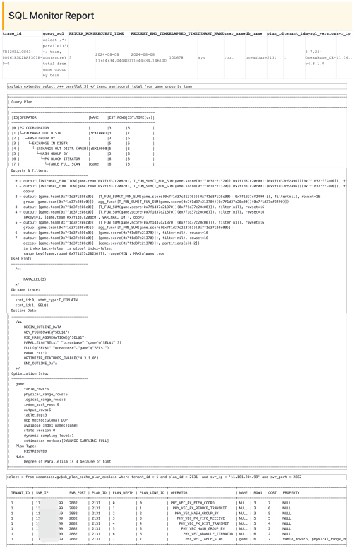
The table headers of the SQL monitor report display the basic SQL execution information obtained from the GV$OB_SQL_AUDIT view.

Execution plan information
The following figure shows the execution plan information.

An execution plan comprises two parts, one of which is the execution result of the EXPLAIN EXTENDED statement, namely, the physical execution plan, which is not the execution plan hit by the SQL statement. The actual execution plan hit is the part after the physical execution plan.
The physical execution plan displays information such as the statistics, hints, and outline data. The physical execution plan and actual execution plan are the same in most cases. If they are not the same, you need to pay attention to the situation.
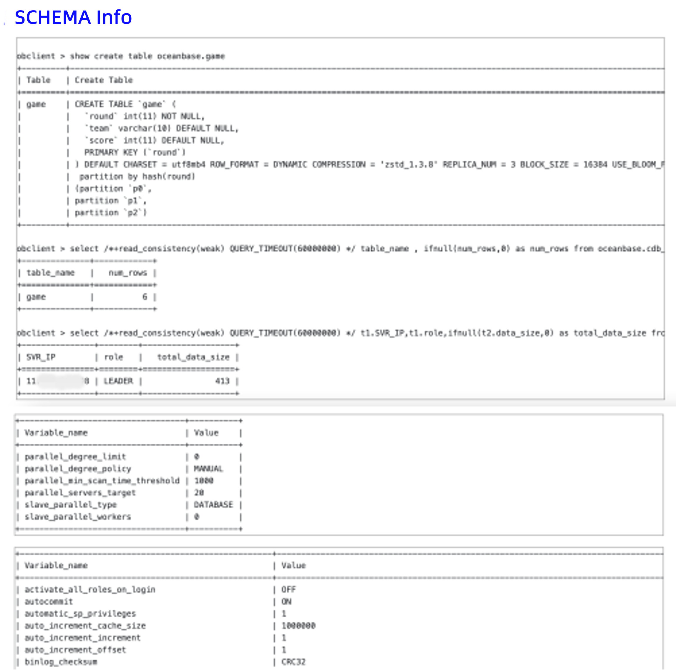
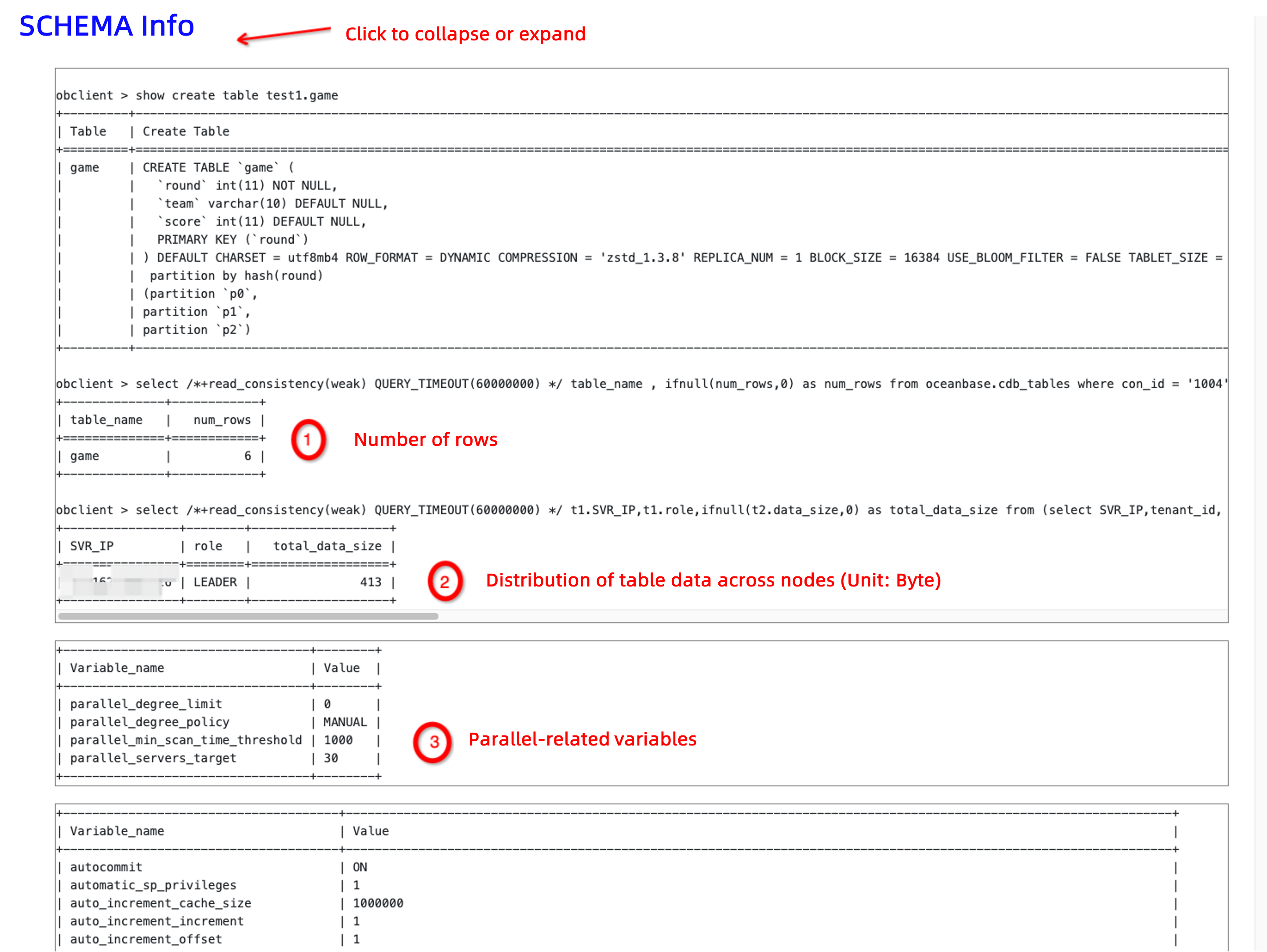
SCHEMA Info
Click SCHEMA Info highlighted in blue to expand and collapse the information. As shown in the following figure, you need to pay attention to whether the number of rows (num_rows) matches the execution result of the EXPLAIN EXTENDED statement. If the order of magnitude has an error, it is probable that a lag exists in statistics collection. In this case, you need to resolve the lag in statistics collection before you handle the issue of slow SQL statements.
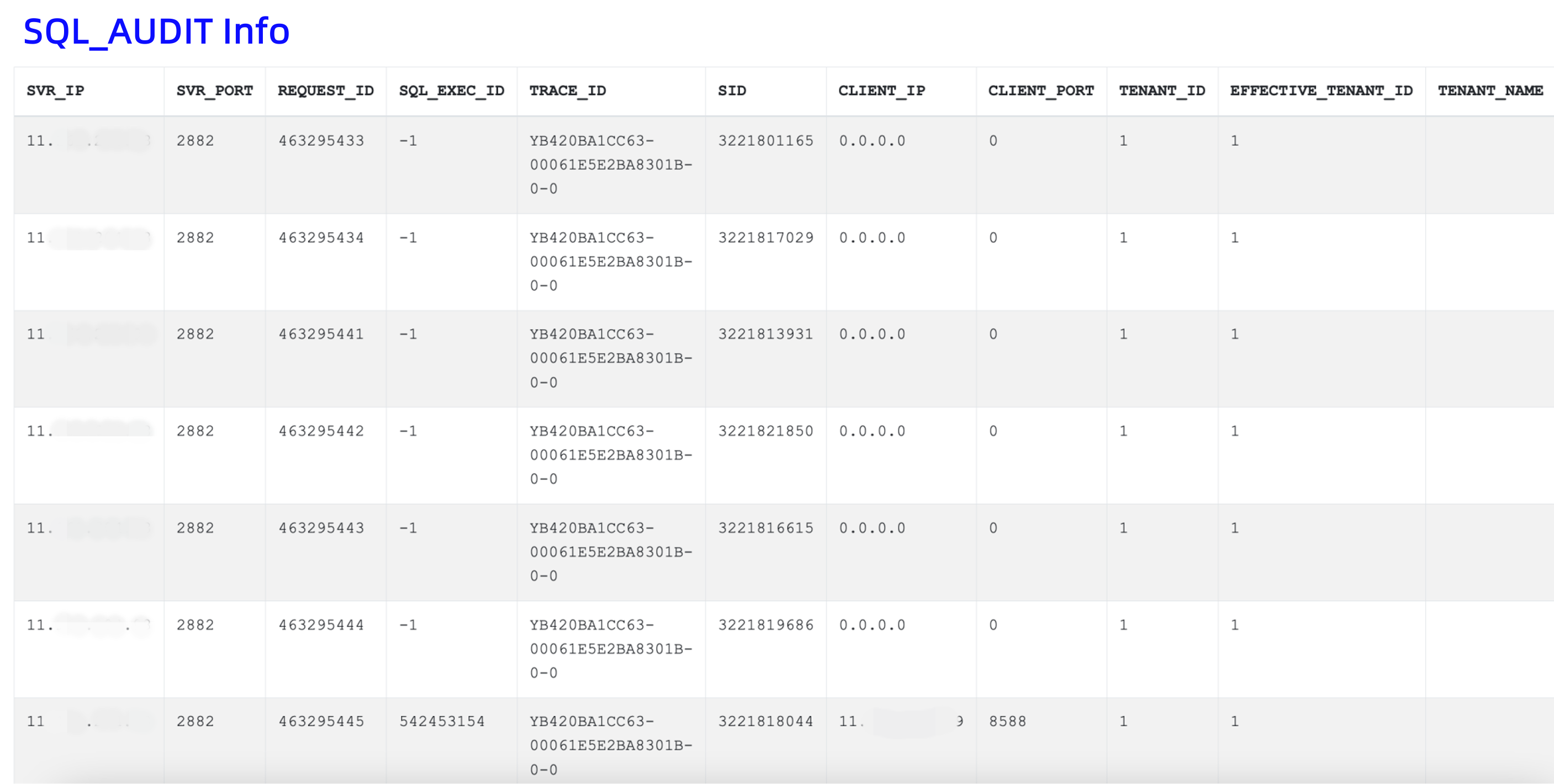
SQL_AUDIT Info
Click SQL_AUDIT Info highlighted in blue to expand and collapse the information.

The used SQL statement is as follows:
-- ob 4.x --
select /*+ sql_audit */
`SVR_IP`,`SVR_PORT`,`REQUEST_ID`,`SQL_EXEC_ID`,`TRACE_ID`,`SID`,`CLIENT_IP`,`CLIENT_PORT`,`TENANT_ID`,
`EFFECTIVE_TENANT_ID`,`TENANT_NAME`,`USER_ID`,`USER_NAME`,`USER_CLIENT_IP`,`DB_ID`,`DB_NAME`,`SQL_ID`,
`QUERY_SQL`,`PLAN_ID`,`AFFECTED_ROWS`,`RETURN_ROWS`,`PARTITION_CNT`,`RET_CODE`,`QC_ID`,`DFO_ID`,`SQC_ID`,
`WORKER_ID`,`EVENT`,`P1TEXT`,`P1`,`P2TEXT`,`P2`,`P3TEXT`,`P3`,`LEVEL`,`WAIT_CLASS_ID`,`WAIT_CLASS`,`STATE`,
`WAIT_TIME_MICRO`,`TOTAL_WAIT_TIME_MICRO`,`TOTAL_WAITS`,`RPC_COUNT`,`PLAN_TYPE`,`IS_INNER_SQL`,
`IS_EXECUTOR_RPC`,`IS_HIT_PLAN`,`REQUEST_TIME`,`ELAPSED_TIME`,`NET_TIME`,`NET_WAIT_TIME`,`QUEUE_TIME`,
`DECODE_TIME`,`GET_PLAN_TIME`,`EXECUTE_TIME`,`APPLICATION_WAIT_TIME`,`CONCURRENCY_WAIT_TIME`,
`USER_IO_WAIT_TIME`,`SCHEDULE_TIME`,`ROW_CACHE_HIT`,`BLOOM_FILTER_CACHE_HIT`,`BLOCK_CACHE_HIT`,
`DISK_READS`,`RETRY_CNT`,`TABLE_SCAN`,`CONSISTENCY_LEVEL`,`MEMSTORE_READ_ROW_COUNT`,
`SSSTORE_READ_ROW_COUNT`,`REQUEST_MEMORY_USED`,`EXPECTED_WORKER_COUNT`,`USED_WORKER_COUNT`,
`TX_ID`,`REQUEST_TYPE`,`IS_BATCHED_MULTI_STMT`,`OB_TRACE_INFO`,`PLAN_HASH`
from oceanbase.gv$ob_sql_audit where trace_id = '%s' " "AND client_ip IS NOT NULL ORDER BY QUERY_SQL ASC, REQUEST_ID
The following figure shows the time consumption in each execution phase of a request.
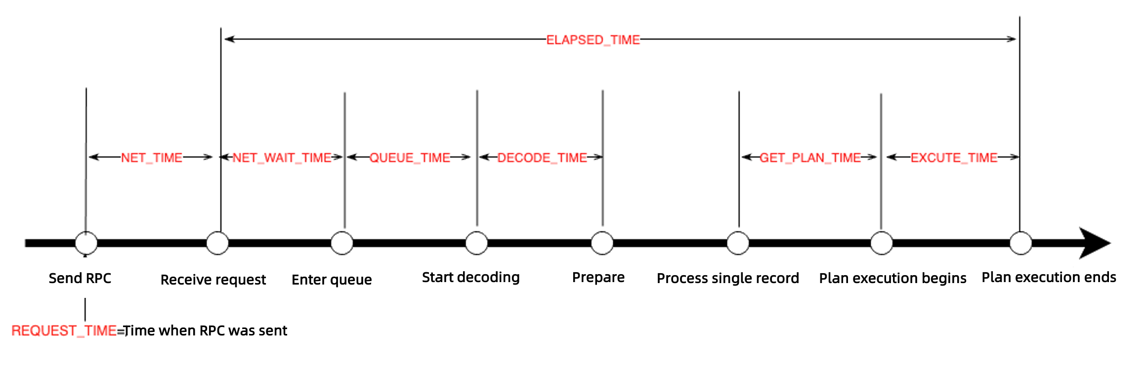
Pay attention to the following fields in the SQL audit information:
PLAN_TYPE: the type of the execution plan for the SQL statement.plan_type=1: indicates that a local execution plan is used, which has the best performance.plan_type=2: indicates that a remote execution plan is used.plan_type=3: indicates that a distributed execution plan is used, including a local execution plan and a remote execution plan.
Generally, a large number of remote execution requests may be the result of a follower-to-leader switchover, or inaccurate routing by OceanBase Database Proxy (ODP).
RETRY_CNT: the number of retries. A large number indicates possible lock contention or follower-to-leader switchover.QUEUE_TIME: the queuing time.GET_PLAN_TIME: the time spent in obtaining the execution plan. A large value of this field is often accompanied byIS_HIT_PLAN = 0, which means that the plan cache is not hit.EXECUTE_TIME: the execution time. If the execution time is long:- Check for time-consuming wait events.
- Check the
SSSTORE_READ_ROW_COUNTandMEMSTORE_READ_ROW_COUNTfields to verify whether a large number of rows are accessed. For example, response time jitters may occur due to different cardinalities.
SQL_PLAN_MONITOR DFO Summary
Click SQL_PLAN_MONITOR DFO Summary highlighted in blue to expand and collapse the information.
The producer-consumer pipeline model can be used for parallel execution. The PX coordinator parses the execution plan into multiple steps. Each step is called a data flow operation (DFO), namely, a subplan. Each DFO contains multiple operators that are executed in serial. For example, one DFO may contain partition scan, aggregate, and send operators. Another DFO may contain collect and aggregate operators.
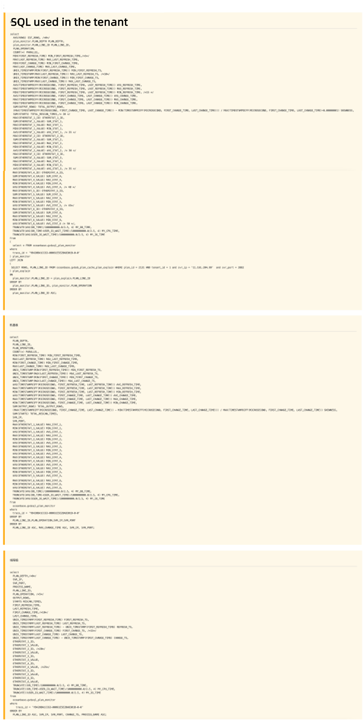
Here is an SQL statement encapsulated by obdiag:
-- DFO level
select
  AVG(ROWS) EST_ROWS, /*0*/
  plan_monitor.PLAN_DEPTH PLAN_DEPTH,
  plan_monitor.PLAN_LINE_ID PLAN_LINE_ID,
  PLAN_OPERATION,
  COUNT(*) PARALLEL,
  MIN(FIRST_REFRESH_TIME) MIN_FIRST_REFRESH_TIME,/*5*/
  MAX(LAST_REFRESH_TIME) MAX_LAST_REFRESH_TIME,
  MIN(FIRST_CHANGE_TIME) MIN_FIRST_CHANGE_TIME,
  MAX(LAST_CHANGE_TIME) MAX_LAST_CHANGE_TIME,
  UNIX_TIMESTAMP(MIN(FIRST_REFRESH_TIME)) MIN_FIRST_REFRESH_TS,
  UNIX_TIMESTAMP(MAX(LAST_REFRESH_TIME)) MAX_LAST_REFRESH_TS, /*10*/
  UNIX_TIMESTAMP(MIN(FIRST_CHANGE_TIME)) MIN_FIRST_CHANGE_TS,
  UNIX_TIMESTAMP(MAX(LAST_CHANGE_TIME)) MAX_LAST_CHANGE_TS,
  AVG(TIMESTAMPDIFF(MICROSECOND, FIRST_REFRESH_TIME, LAST_REFRESH_TIME)) AVG_REFRESH_TIME,
  MAX(TIMESTAMPDIFF(MICROSECOND, FIRST_REFRESH_TIME, LAST_REFRESH_TIME)) MAX_REFRESH_TIME,
  MIN(TIMESTAMPDIFF(MICROSECOND, FIRST_REFRESH_TIME, LAST_REFRESH_TIME)) MIN_REFRESH_TIME, /*15 */
  AVG(TIMESTAMPDIFF(MICROSECOND, FIRST_CHANGE_TIME, LAST_CHANGE_TIME)) AVG_CHANGE_TIME,
  MAX(TIMESTAMPDIFF(MICROSECOND, FIRST_CHANGE_TIME, LAST_CHANGE_TIME)) MAX_CHANGE_TIME,
  MIN(TIMESTAMPDIFF(MICROSECOND, FIRST_CHANGE_TIME, LAST_CHANGE_TIME)) MIN_CHANGE_TIME,
  SUM(OUTPUT_ROWS) TOTAL_OUTPUT_ROWS,
  (MAX(TIMESTAMPDIFF(MICROSECOND, FIRST_CHANGE_TIME, LAST_CHANGE_TIME)) - MIN(TIMESTAMPDIFF(MICROSECOND, FIRST_CHANGE_TIME, LAST_CHANGE_TIME))) / MAX(TIMESTAMPDIFF(MICROSECOND, FIRST_CHANGE_TIME, LAST_CHANGE_TIME)+0.00000001) SKEWNESS,
  SUM(STARTS) TOTAL_RESCAN_TIMES,/* 20 */
  MAX(OTHERSTAT_1_ID) OTHERSTAT_1_ID,
  SUM(OTHERSTAT_1_VALUE) SUM_STAT_1,
  MAX(OTHERSTAT_1_VALUE) MAX_STAT_1,
  MIN(OTHERSTAT_1_VALUE) MIN_STAT_1,
  AVG(OTHERSTAT_1_VALUE) AVG_STAT_1, /* 25 */
  MAX(OTHERSTAT_2_ID) OTHERSTAT_2_ID,
  SUM(OTHERSTAT_2_VALUE) SUM_STAT_2,
  MAX(OTHERSTAT_2_VALUE) MAX_STAT_2,
  MIN(OTHERSTAT_2_VALUE) MIN_STAT_2,
  AVG(OTHERSTAT_2_VALUE) AVG_STAT_2, /* 30 */
  MAX(OTHERSTAT_3_ID) OTHERSTAT_3_ID,
  SUM(OTHERSTAT_3_VALUE) SUM_STAT_3,
  MAX(OTHERSTAT_3_VALUE) MAX_STAT_3,
  MIN(OTHERSTAT_3_VALUE) MIN_STAT_3,
  AVG(OTHERSTAT_3_VALUE) AVG_STAT_3, /* 35 */
  MAX(OTHERSTAT_4_ID) OTHERSTAT_4_ID,
  SUM(OTHERSTAT_4_VALUE) SUM_STAT_4,
  MAX(OTHERSTAT_4_VALUE) MAX_STAT_4,
  MIN(OTHERSTAT_4_VALUE) MIN_STAT_4,
  AVG(OTHERSTAT_4_VALUE) AVG_STAT_4, /* 40 */
  MAX(OTHERSTAT_5_ID) OTHERSTAT_5_ID,
  SUM(OTHERSTAT_5_VALUE) SUM_STAT_5,
  MAX(OTHERSTAT_5_VALUE) MAX_STAT_5,
  MIN(OTHERSTAT_5_VALUE) MIN_STAT_5,
  AVG(OTHERSTAT_5_VALUE) AVG_STAT_5, /* 45*/
  MAX(OTHERSTAT_6_ID) OTHERSTAT_6_ID,
  SUM(OTHERSTAT_6_VALUE) SUM_STAT_6,
  MAX(OTHERSTAT_6_VALUE) MAX_STAT_6,
  MIN(OTHERSTAT_6_VALUE) MIN_STAT_6,
  AVG(OTHERSTAT_6_VALUE) AVG_STAT_6 /* 50 */,
  TRUNCATE(AVG(DB_TIME)/1000000000.0/2.5, 4) MY_DB_TIME,
  TRUNCATE(AVG(DB_TIME-USER_IO_WAIT_TIME)/1000000000.0/2.5, 4) MY_CPU_TIME,
  TRUNCATE(AVG(USER_IO_WAIT_TIME)/1000000000.0/2.5, 4) MY_IO_TIME
from
(
  select * FROM oceanbase.gv$sql_plan_monitor
where
  trace_id = 'YF2A0BA2DA7E-00061D6A8ADDA95A-0-0'
) plan_monitor
LEFT JOIN
(
 SELECT ROWS, PLAN_LINE_ID FROM oceanbase.gv$ob_plan_cache_plan_explain WHERE plan_id = xxx AND tenant_id = xxxx and svr_ip = 'xxxx'  and svr_port = xxxx
) plan_explain
ON
  plan_monitor.PLAN_LINE_ID = plan_explain.PLAN_LINE_ID
GROUP BY
  plan_monitor.PLAN_LINE_ID, plan_monitor.PLAN_OPERATION
ORDER BY
  plan_monitor.PLAN_LINE_ID ASC;
SQL_PLAN_MONITOR SQC Summary
Click SQL_PLAN_MONITOR SQC Summary highlighted in blue to expand and collapse the information.
The concepts involved in this part are described as follows:
QC: short for query coordinator. When you execute an SQL statement to query data on two or more OBServer nodes or query a partitioned table on a single OBServer node, the statement is executed in parallel. When the SQL plan encounters a parallel query on the OBServer node that you connect to, the main process determines the degree of parallelism (DOP) and schedules worker threads to process requests on various OBServer nodes. The OBServer node that you connect to acts as the QC.
SQC: short for subquery coordinator. Each thread that processes a QC request is naturally an SQC of this query. An SQC is responsible for preparing resources and context for DFOs on each OBServer node. After that, DFOs are executed in parallel on the OBServer nodes.
SQL_PLAN_MONITOR Details
Click SQL_PLAN_MONITOR Details highlighted in blue to expand and collapse the information.
This part provides information about operators and threads. You can check the operators and threads with a long execution time. You can also check idle threads. If most threads are idle, parallel execution cannot achieve the expected effect. In this case, you need to check whether the parallel execution settings are correct.
Case study: An incorrect execution plan is selected due to inaccurate statistics
Here is the information about an SQL statement executed in the actual business scenario:
SELECT
    `t`.`date` AS `date`,
    SUM(`t`.`adcost`) AS `adcost`,
    SUM(`t`.`ns`) AS `ns`,
    SUM(`t`.`nc`) AS `nc`,
    SUM(`t`.`realtimeordernum`) AS `realtimeordernum`,
    SUM(`t`.`realtimeorderprice`) AS `realtimeorderprice`
FROM
    (select * from `galileo`.`report_game_consume_conversion` where `date` BETWEEN '2024-07-21' AND '2024-07-22') AS `t`
        JOIN (
        SELECT
            `date` AS `date1`,
            `solutionid`
        FROM
            `galileo`.`report_game_solution`
        WHERE
            `date` BETWEEN '2024-07-21' AND '2024-07-22'
    ) AS `t1` ON `t1`.`date1`=`t`.`date`
        AND `t`.`solutionid`=`t1`.`solutionid`
        JOIN (
        SELECT
            `date` AS `date2`,
            `adspaceid`
        FROM
            `galileo`.`report_game_adspace`
        WHERE
            `date` BETWEEN '2024-07-21' AND '2024-07-22'
    ) AS `t2` ON `t2`.`date2`=`t`.`date`
        AND `t`.`adspaceid`=`t2`.`adspaceid`
        LEFT JOIN (
        SELECT
            `date` AS `date3`,
            `solutionid`,
            `adspaceid`
        FROM
            `galileo`.`report_game_order`
        WHERE
            `date` BETWEEN '2024-07-21' AND '2024-07-22'
        GROUP BY
            `date`,
            `solutionid`,
            `adspaceid`
    ) AS `t3` ON `t3`.`date3`=`t`.`date`
        AND `t`.`solutionid`=`t3`.`solutionid`
        AND `t`.`adspaceid`=`t3`.`adspaceid`
GROUP BY
    `t`.`date` limit 10
It was found that the execution of the SQL statement was slow. Therefore, the aforesaid method was used to collect SQL diagnostic information. Here is a screenshot of the collection report:
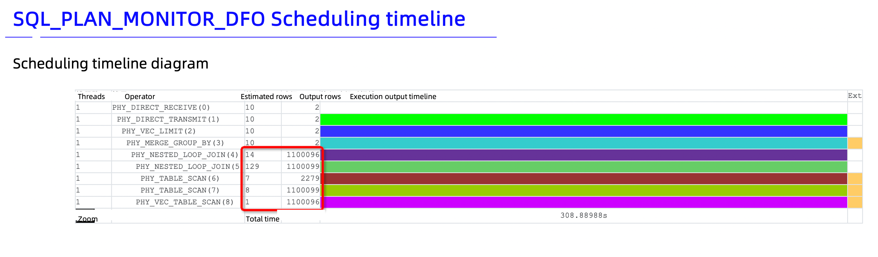
The collection report shows that the number of estimated rows differs greatly from the number of output rows. The schema information in the report shows that millions of data rows exist. This proves that the number of output rows is accurate but the number of estimated rows is not. Inaccurate estimation easily misleads the optimizer, which will thus select an incorrect execution plan.
The diagnostic information shows that the execution plan contains three PHY_NESTED_LOOP_JOIN operators. A query on any of the three tables returns millions of rows. Using PHY_NESTED_LOOP_JOIN operators is time-consuming. A hash join is a better choice in this case.
It is found that a multi-table join was performed. A hint can be used to adjust the operators.
/*+
LEADING(@"SEL$1" (("galileo"."report_game_solution"@"SEL$3" "galileo"."report_game_consume_conversion"@"SEL$2") "galileo"."report_game_adspace"@"SEL$4"))
USE_HASH(@"SEL$1" "galileo"."report_game_adspace"@"SEL$4")                                                                                                                                                            |
USE_HASH(@"SEL$1" "galileo"."report_game_consume_conversion"@"SEL$2")
*/
Note
For more information about hints, see Optimizer hints.
If you do not know how to specify a hint, see the execution result of the EXPLAIN EXTENDED statement and modify the result based on the actual situation.

After a hint is specified, the execution result is returned within 4s, which is much shorter than the original 300s. The hint significantly improves the query performance.
References
For more information about obdiag, see obdiag documentation.