


An execution plan describes the process of executing an SQL query statement in OceanBase Database. You can run the EXPLAIN command to view the logical execution plan generated by the optimizer for a given SQL statement.
To analyze the performance of an SQL statement, you need to first check the SQL execution plan to see if any error exists. Therefore, understanding the execution plan is the first step for SQL optimization, and knowledge about operators of an execution plan is key to understanding the EXPLAIN command.
Syntax of the EXPLAIN command
OceanBase Database supports three EXPLAIN command formats: EXPLAIN BASIC, EXPLAIN, and EXPLAIN EXTENDED. They demonstrate details of execution plans at different levels:
The
EXPLAIN BASICcommand shows the most basic framework of a plan.The
EXPLAIN EXTENDEDcommand extends a plan to its full frame with the most details and is usually used in troubleshooting.The
EXPLAINcommand shows information to the extent that helps users understand the entire execution process of a plan.
Format of command:
EXPLAIN [BASIC | EXTENDED | PARTITIONS | FORMAT = format_name] explainable_stmt
format_name:
  { TRADITIONAL | JSON }
explainable_stmt:
  { SELECT statement
 | DELETE statement
 | INSERT statement
 | REPLACE statement
 | UPDATE statement }
Shape and operators of an execution plan
In a database system, an execution plan is usually represented in a tree-like structure. However, different databases display execution plans in different ways.
The following examples show the execution plans for TPC-DS Q3 in PostgreSQL, Oracle, and OceanBase Database.
obclient> SELECT /*TPC-DS Q3*/ *
     FROM (SELECT dt.d_year,
                  item.i_brand_id    brand_id,
                  item.i_brand       brand,
                  Sum(ss_net_profit) sum_agg
           FROM   date_dim dt,
                  store_sales,
                  item
           WHERE  dt.d_date_sk = store_sales.ss_sold_date_sk
                  AND store_sales.ss_item_sk = item.i_item_sk
                  AND item.i_manufact_id = 914
                  AND dt.d_moy = 11
           GROUP  BY dt.d_year,
                  item.i_brand,
                  item.i_brand_id
           ORDER  BY dt.d_year,
                  sum_agg DESC,
                  brand_id)
     WHERE ROWNUM <= 100;
Execution plan in PostgreSQL:
Limit  (cost=13986.86..13987.20 rows=27 width=91)
         Sort  (cost=13986.86..13986.93 rows=27 width=65)
         Sort Key: dt.d_year, (sum(store_sales.ss_net_profit)), item.i_brand_id
              HashAggregate  (cost=13985.95..13986.22 rows=27 width=65)
                     Merge Join  (cost=13884.21..13983.91 rows=204 width=65)
                     Merge Cond: (dt.d_date_sk = store_sales.ss_sold_date_sk)
                           Index Scan using date_dim_pkey on date_dim dt  (cost=0.00..3494.62 rows=6080 width=8)
                           Filter: (d_moy = 11)
                           Sort  (cost=12170.87..12177.27 rows=2560 width=65)
                           Sort Key: store_sales.ss_sold_date_sk
                                 Nested Loop  (cost=6.02..12025.94 rows=2560 width=65)
                                       Seq Scan on item  (cost=0.00..1455.00 rows=16 width=59)
                                       Filter: (i_manufact_id = 914)
                                       Bitmap Heap Scan on store_sales  (cost=6.02..658.94 rows=174 width=14)
                                       Recheck Cond: (ss_item_sk = item.i_item_sk)
                                             Bitmap Index Scan on store_sales_pkey  (cost=0.00..5.97 rows=174 width=0)
                                             Index Cond: (ss_item_sk = item.i_item_sk)
Execution plan in Oracle:
Plan hash value: 2331821367
----------------------------------------------------------------------------
| Id  | Operation                         | Name         | Rows  | Bytes | Cost (%CPU)| Time     |
----------------------------------------------------------------------------
|   0 | SELECT STATEMENT                  |              |   100 |  9100 |  3688   (1)| 00:00:01 |
|*  1 |  COUNT STOPKEY                    |              |       |       |            |          |
|   2 |   VIEW                            |              |  2736 |   243K|  3688   (1)| 00:00:01 |
|*  3 |    SORT ORDER BY STOPKEY          |              |  2736 |   256K|  3688   (1)| 00:00:01 |
|   4 |     HASH GROUP BY                 |              |  2736 |   256K|  3688   (1)| 00:00:01 |
|*  5 |      HASH JOIN                    |              |  2736 |   256K|  3686   (1)| 00:00:01 |
|*  6 |       TABLE ACCESS FULL           | DATE_DIM     |  6087 | 79131 |   376   (1)| 00:00:01 |
|   7 |       NESTED LOOPS                |              |  2865 |   232K|  3310   (1)| 00:00:01 |
|   8 |        NESTED LOOPS               |              |  2865 |   232K|  3310   (1)| 00:00:01 |
|*  9 |         TABLE ACCESS FULL         | ITEM         |    18 |  1188 |   375   (0)| 00:00:01 |
|* 10 |         INDEX RANGE SCAN          | SYS_C0010069 |   159 |       |     2   (0)| 00:00:01 |
|  11 |        TABLE ACCESS BY INDEX ROWID| STORE_SALES  |   159 |  2703 |   163   (0)| 00:00:01 |
--------------------------------------------------------------------------------------------------
Execution plan in OceanBase Database:
|ID|OPERATOR              |NAME       |EST. ROWS|COST |
-------------------------------------------------------
|0 |LIMIT                 |           |100      |81141|
|1 | TOP-N SORT           |           |100      |81127|
|2 |  HASH GROUP BY       |           |2924     |68551|
|3 |   HASH JOIN          |           |2924     |65004|
|4 |    SUBPLAN SCAN      |VIEW1      |2953     |19070|
|5 |     HASH GROUP BY    |           |2953     |18662|
|6 |      NESTED-LOOP JOIN|           |2953     |15080|
|7 |       TABLE SCAN     |ITEM       |19       |11841|
|8 |       TABLE SCAN     |STORE_SALES|161      |73   |
|9 |    TABLE SCAN        |DT         |6088     |29401|
=======================================================
You may notice from the foregoing examples that a plan in OceanBase Database is similar to that in Oracle Database.
The following table describes columns of an execution plan in OceanBase Database.
Column name |
Description |
|---|---|
ID |
The sequence number of the execution tree obtained by using preorder traversal, starting from 0. |
OPERATOR |
The name of the operator. |
NAME |
The name of the table or index corresponding to a table operation. |
EST. ROWS |
The estimated number of output rows of the operator. |
COST |
The execution cost of the operator, in µs. |
Note
In a table operation, the
NAMEfield displays names (aliases) of tables involved in the operation. In the case of index access, the name of the index is displayed in parentheses after the table name. For example,t1(t1_c2)indicates that indext1_c2is used. In the case of reverse scanning, the keywordRESERVEis added after the index name, with the index name and the keyword RESERVE separated with a comma (,), such ast1(t1_c2,RESERVE).
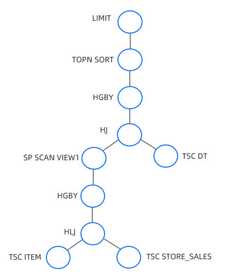
In OceanBase Database, the first part of the output of the EXPLAIN command is the tree structure of the execution plan. The hierarchy of operations in the tree is represented by their indentations in the operator column. Operators at the deepest level are executed first. Operators at the same level are executed in the specified execution order.
The following figure shows the tree structure of the plan in the TPCDS Q3 example.
In OceanBase Database, the second part of the output of the EXPLAIN command contains the details of each operator, including the output expression, filter conditions, partition information, and unique information of each operator, such as the sort keys, join keys, and pushdown conditions. For example:
Outputs & filters:
-------------------------------------
  0 - output([t1.c1], [t1.c2], [t2.c1], [t2.c2]), filter(nil), sort_keys([t1.c1, ASC], [t1.c2, ASC]), prefix_pos(1)
  1 - output([t1.c1], [t1.c2], [t2.c1], [t2.c2]), filter(nil),
      equal_conds([t1.c1 = t2.c2]), other_conds(nil)
  2 - output([t2.c1], [t2.c2]), filter(nil), sort_keys([t2.c2, ASC])
  3 - output([t2.c2], [t2.c1]), filter(nil),
      access([t2.c2], [t2.c1]), partitions(p0)
  4 - output([t1.c1], [t1.c2]), filter(nil),
      access([t1.c1], [t1.c2]), partitions(p0)
For more information about execution plans, see Execution plan operators.