


OceanBase Database provides several vector index algorithms. You can select the most suitable index type based on your specific use case.
Notice
The practices in this document apply only to OceanBase Database V4.3.5 BP3 and later versions.
HNSW or IVF?
OceanBase Database offers two main categories of dense indexes:
- The graph-based HNSW series: HNSW, HNSW_SQ, and HNSW_BQ.
- The disk-based IVF series: IVF and IVF_PQ.
Each index type has its own strengths. The HNSW series typically delivers higher query performance but requires more resident memory. The IVF series performs well when enough cache is available and can operate without needing to reside in memory. However, the choice between HNSW and IVF depends not only on memory usage, but also on your business scenario, data size, performance requirements, and resource constraints. The following sections compare their key differences and offer selection advice.
Key differences
Dimension |
HNSW series |
IVF series |
|---|---|---|
| Storage method | Memory-based graph structure index | Disk-based index |
| Memory usage | Must be fully loaded into memory; high memory usage | Can run without resident memory; low memory usage |
| Query performance (QPS) | Extremely high; millisecond-level response | High; nearly matches HNSW when cache is sufficient |
| Recall rate | High, up to 99% | High, slightly lower than HNSW; can be tuned with parameters |
| Build speed | Slower; requires graph construction | Faster; uses clustering algorithms |
| Suitable data volume | Millions to hundreds of millions | Millions to billions |
| Cost | High memory cost | Low storage cost; ideal for large-scale data |
| Real-time capability | Supports real-time DML operations | Supports real-time DML operations |
Decision flowchart
Note
- Before choosing an index type, please refer to vector index memory management to estimate memory requirements.
- The recommendations in the flowchart are based on 1024-dimensional vectors. For vectors with different dimensions, adjust resource estimates proportionally.
- The flowchart mainly considers memory cost to help guide your decision.
- Even if tenant memory is sufficient, you do not always need to choose the highest-spec index such as HNSW. If you want excellent performance with better cost efficiency, consider options like HNSW_SQ.
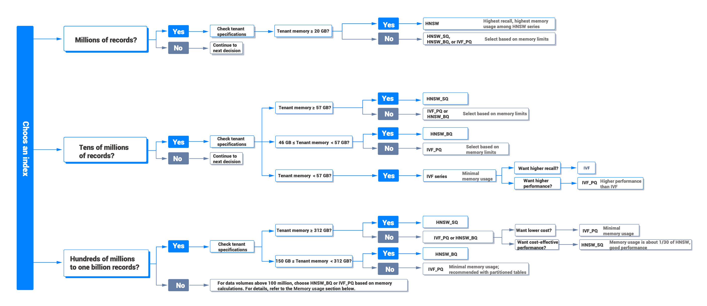
Notice
This flowchart illustrates only common scenarios. If your situation is not covered, or if you have special requirements, please contact OceanBase technical support.
Use partitioned tables?
Partitioned tables are mainly recommended for handling very large datasets. If your query conditions can be mapped to a partition key, partition pruning can further improve query performance. Consider partitioned tables in these scenarios:
- When your dataset reaches tens of millions or hundreds of millions of records: Partitioning distributes data across multiple partitions, allowing each partition to build its own index. This reduces the load per query and improves overall performance.
- When your query conditions include a scalar column suitable for partition pruning: For example, if the
labelfield is always present in theWHEREclause, you can uselabelas the partition key. Partition pruning reduces the number of partitions that need to be scanned.
Recommended practices:
Partitioning
When using vector indexes, avoid excessive partitioning. Unlike scalar indexes, vector indexes (such as HNSW) do not significantly increase TopK query computation cost when scaling from 1 million to 2 million vectors. If partition pruning is not possible, too many partitions may actually hurt performance. Conversely, overly large partitions can slow down index rebuilding and reduce efficiency in queries that combine scalar and vector conditions.
In summary, it is recommended to keep the data volume per partition below 20 million records, and to choose partition keys that support partition pruning.
Algorithm selection
For large datasets, HNSW_BQ or IVF_PQ indexes are recommended. For other index types, refer to the Memory usage section below for sizing guidance.
Memory usage
HNSW_BQ
For the HNSW_BQ index, we recommend that tenant memory > total memory required for HNSW_BQ queries + memory required for a single partition's HNSW_SQ index. The memory estimation process is as follows:
- Use the
INDEX_VECTOR_MEMORY_ADVISORfunction to calculate recommended memory for both HNSW_BQ and HNSW_SQ during index building and querying. - Based on the recommended values, determine the total memory required for the tenant.
For example, with 100 million 1024-dimensional vectors and 10 partitions (about 10 million vectors per partition):
-- Specify REFINE_TYPE=SQ8 to accurately estimate memory usage for HNSW_BQ during both index building and querying.
-- No need to separately calculate memory usage for HNSW_SQ, as HNSW_BQ uses SQ8 quantization by default.
-- After specifying refine_type=sq8, the function automatically includes the memory required for the SQ8 quantized vectors in the calculation.
-- For HNSW_BQ, the recommended memory is 74.6 GB; memory usage during query is 57.4 GB. Use the recommended value.
SELECT DBMS_VECTOR.INDEX_VECTOR_MEMORY_ADVISOR('HNSW_BQ',100000000,1024,'FLOAT32','M=32,DISTANCE=COSINE,REFINE_TYPE=SQ8', 10000000);
+------------------------------------------------------------------------------------------------------------------------------+
| DBMS_VECTOR.INDEX_VECTOR_MEMORY_ADVISOR('HNSW_BQ',100000000,1024,'FLOAT32','M=32,DISTANCE=COSINE,REFINE_TYPE=SQ8', 10000000) |
+------------------------------------------------------------------------------------------------------------------------------+
| Suggested minimum vector memory is 74.6 GB, memory consumption when providing search service is 57.4 GB |
+------------------------------------------------------------------------------------------------------------------------------+
1 row in set
-- The default proportion of vector memory in tenant memory is 50%. Therefore, the total tenant memory is:
SELECT 74.6/0.5;
+--------------------------------------------------------------------------------------------------------------+
| 74.6/0.5 = 149.2 GB |
+--------------------------------------------------------------------------------------------------------------+
1 row in set
-- Considering that new data may not be compressed in actual environments, we recommend reserving some redundancy.
SELECT 149.2 * 1.2;
+--------------------------------------------------------------------------------------------------------------+
| 149.2 * 1.2 = 179.04 GB |
+--------------------------------------------------------------------------------------------------------------+
1 row in set
-- Therefore, we recommend configuring the tenant memory to 179 GB.
IVF series
For IVF and IVF_PQ indexes, it is recommended that tenant memory > memory required for constructing a single partition + total memory required for all partitions. For example, with 100 million records and 10 partitions (about 10 million vectors per partition), building a single partition requires about 2.7 GB memory, and total resident memory for 10 IVF_PQ partitions is about 1.1 GB (110 MB per partition). So the minimum configuration is about 3 GB. It is recommended to allow extra buffer and configure 6 GB tenant memory. For other dataset sizes, estimate accordingly.
Build and query parameters
Set index build and query parameters based on the maximum data volume per partition. For details, see the Index parameter recommendations section below.
Performance and recall rate
- If queries can be limited to a single partition: Performance and recall match single-partition scenarios; see below for details by data scale.
- If queries cannot be limited to a single partition: QPS can be estimated by dividing single-partition performance by the number of partitions per OBServer node (for example, 3 partitions per node means QPS is roughly one-third of single-partition QPS). Cross-partition queries aggregate more candidates, so recall is often higher than in single-partition cases.
Index parameter recommendations
HNSW series
Recommended build and query parameters vary by data volume. This section provides suggested configurations for 768-dimensional vectors with 1 million and 10 million records, for HNSW, HNSW_SQ, and HNSW_BQ indexes. For datasets of 100 million records or more, use IVF_PQ or HNSW_BQ with partitioned tables.
Notice
FIf your data volume is expected to grow, set parameters according to the final expected size.
Notice
HNSW_BQ uses a high-compression quantization algorithm, and its recall ceiling may be lower for low-dimensional vectors. To avoid performance loss, use HNSW_BQ for vectors with 512 dimensions or higher.
Scenario |
Index type |
Recommended parameters |
|---|---|---|
| Maximum recall (Highest memory usage) |
HNSW | 1M records: m = 16, ef_construction = 200, ef_search = 100, other parameters default |
| Maximum performance (Lower memory usage) |
HNSW_SQ | 1M records: m = 16, ef_construction = 200, ef_search = 100, other parameters default 10M records: m = 32, ef_construction = 400, ef_search = 350, other parameters default |
| Best cost-performance (Low memory, good performance) |
HNSW_BQ | 1M records: m = 16, ef_construction = 200, ef_search = 100, other parameters default 10M records: m = 32, ef_construction = 400, ef_search = 1000, refine_k = 10, other parameters default 100M records: use partitioned tables, m = 32, ef_construction = 400, ef_search = 1000, refine_k = 10, other parameters default |
Details for datasets with one million records
Let's take one million 768-dimensional vectors as an example (using the recommended parameters above) to explain memory usage and recall optimization:
Memory usage:
Index type |
Recommended tenant memory |
Description |
|---|---|---|
| HNSW | 15 GB | The recommended memory for the vector index is 7.3 GB. When tenant memory exceeds 8 GB, vector indexes can use up to 50% of the available memory by default; if tenant memory is 8 GB or less, they use up to 40%. So you will need around 15 GB of tenant memory. |
| HNSW_SQ | 6 GB | The recommended memory for the vector index is 2.1 GB. |
| HNSW_BQ | 6 GB | Building an HNSW_BQ index requires high-precision vectors, so its memory needs during construction are the same as HNSW_SQ—6 GB. By default, HNSW_BQ uses the SQ8 quantization method, which significantly reduces memory usage after the index is built, down to about 405 MB. This applies to non-partitioned tables. If you’re using partitioned tables, OceanBase Database will automatically adjust how many partitions can be built at once based on the tenant's memory allocation. In practice, it is best to allocate enough memory to cover both the memory needed for HNSW_BQ queries and the memory required to build HNSW_SQ for a single partition, plus a safety buffer. For specifics, see the Memory usage section above. |
Recall optimization:
You can boost recall by increasing the ef_search and refine_k parameters (refine_k is only for HNSW_BQ). Higher values mean more vector computations and better recall, but slower query performance. For different TopN results, use the recommended values below. If you need even higher recall, you can set these parameters even higher.
Notice
Recall is closely tied to your data characteristics. The table below shows values recommended for a standard 768-dimensional dataset to achieve about 0.95 recall.
TopN |
ef_search |
refine_k (HNSW_BQ only) |
|---|---|---|
| Top10 | 64 | 4 |
| Top100 | 240 | 4 |
About maximum recall:
Each index algorithm has a different upper limit for recall. With the recommended parameters above, setting ef_search to 1000 can further improve recall, but QPS (queries per second) will drop to about one-third of what you get at 0.95 recall. Also, simply increasing ef_search does not always keep improving recall for every index type—only HNSW can reach recall rates above 0.99. For HNSW_BQ, you can increase refine_k for even better recall, but this will further reduce performance.
Reference values for maximum recall (ef_search = 1000):
- HNSW: recall 0.991
- HNSW_SQ: recall 0.9786
- HNSW_BQ: recall 0.9897 (
ef_search= 1000,refine_k= 10)
Details for datasets with ten million records
Now let's look at ten million 768-dimensional vectors (again, using the recommended parameters) to explain memory usage and recall optimization:
Memory usage:
Index type |
Recommended tenant memory |
Description |
|---|---|---|
| HNSW | 160 GB | The recommended memory for the vector index is 76.3 GB. |
| HNSW_SQ | 48 GB | The recommended memory for the vector index is 22.6 GB. |
| HNSW_BQ | 48 GB | Building HNSW_BQ requires high-precision vectors, and it uses HNSW_SQ as a cache during index construction. For non-partitioned tables, HNSW_BQ needs the same memory as HNSW_SQ. After building, HNSW_BQ only occupies about 5.4 GB of memory. |
Recall optimization:
You can improve recall by adjusting ef_search and refine_k (only for HNSW_BQ). Higher values mean more computation and better recall, but slower queries. For different TopN results, use the recommended settings below. For even higher recall, use larger values.
Notice
Recall is closely tied to your data characteristics. The table below shows values recommended for a standard 768-dimensional dataset to achieve about 0.95 recall.
TopN |
ef_search |
refine_k (HNSW_BQ only) |
|---|---|---|
| Top10 | 100 | 4 |
| Top100 (HNSW/HNSW_SQ) | 350 | - |
| Top100 (HNSW_BQ) | 1000 | 10 |
IVF series
Scenario |
Index type |
Recommended parameters |
|---|---|---|
| Low dimension (384 or fewer) |
IVF | Ten million records: use partitioned tables, nlist = 3000 Hundred million records: use partitioned tables, nlist = 3000 |
| Low cost (Minimal memory) |
IVF_PQ | One million records: nlist = 1000, m = half the vector dimension Ten million records: nlist = 3000, m = half the vector dimension Hundred million records: use partitioned tables, nlist = 3000, m = half the vector dimension |
To balance the number of cluster centers and the amount of data per center, nlist is usually set to the square root of the data size. For ten million records, nlist is typically set to around 3000. For IVF_PQ, it is recommended to set m to half the vector dimension.
Notice
IVF_PQ uses a high-compression quantization algorithm, and its recall ceiling may be lower for low-dimensional vectors. To avoid performance loss, it is best to use IVF_PQ for vectors with at least 128 dimensions.
Notice
If your data volume is expected to grow, set parameters based on the final expected size.
Ten million records (with partitioned tables)
Let's use ten million 768-dimensional vectors as an example (with the recommended parameters) to explain memory usage and recall optimization:
Memory usage:
Index type |
Index parameters |
Memory usage (build/resident) |
|---|---|---|
| IVF | distance = l2, nlist = 3000 | 2.7 GB / 10.5 MB |
| IVF_PQ | distance = l2, nlist = 3000, m = 384 | 4.0 GB / 1.3 GB |
| IVF_PQ | distance = cosine, nlist = 3000, m = 384 | 2.7 GB / 11.4 MB |
Build usage refers to the temporary memory used during index creation, which is released after the index is built. Resident usage is the memory occupied by the index once it is finished and in use.
For IVF_PQ, if you choose distance = l2, more resident memory is required because it stores extra precomputed results. In contrast, using distance = inner_product or cosine uses much less resident memory. In practice, inner_product or cosine are usually preferred to optimize memory usage.
Recall optimization:
You can boost recall by increasing the nprobes parameter, but doing so will reduce query performance. For different TopN results, use the recommended values below. If you want even higher recall, you can set nprobes higher.
Notice
Recall is closely tied to your data characteristics. The table below shows values recommended for a standard 768-dimensional dataset to achieve about 0.95 recall.
TopN |
nprobes |
|---|---|
| Top10 | 1 |
| Top100 | 20 |
Hundred million records (with partitioned tables)
For vector datasets of hundreds of millions or more, we strongly recommend using partitioned tables with IVF indexes. As data size and nlist increase, the query cost for a single IVF index rises sharply. Partitioning splits the data into multiple smaller IVF indexes, reducing the load per query and improving overall performance and recall through parallel queries.
For partitioned tables, each partition maintains its own local IVF index. We recommend calculating nlist based on the average data volume per partition. For example, with 100 million 768-dimensional vectors split into 10 partitions (10 million per partition), set nlist to about sqrt(10 million) ≈ 3162.
Let's use 100 million 768-dimensional vectors as an example (with the recommended parameters) to explain memory usage and recall optimization:
Memory usage:
For partitioned tables, total resident memory is the sum across all partitions. For example, if a single IVF index uses 10.5 MB, then 10 partitions will use about 105 MB in total.
Index type |
Index parameters |
Memory usage (build/resident) |
|---|---|---|
| IVF | distance = l2, nlist = 3000 | 2.7 GB / 10.5 × 10 MB |
| IVF_PQ | distance = l2, nlist = 3000, m = 384 | 4.0 GB / 1.3 × 10 GB |
| IVF_PQ | distance = cosine, nlist = 3000, m = 384 | 2.7 GB / 11.4 × 10 MB |
Build usage refers to the temporary memory used during index creation, which is released after building. Resident usage is the memory occupied by the finished IVF index.
Recall optimization:
You can boost recall by increasing the nprobes parameter, but this will reduce query performance. For different TopN results, use the recommended values below. If you want even higher recall, you can set nprobes higher.
With partitioned tables, each partition runs its own IVF index query. If your search spans multiple partitions, TopN results are retrieved from each partition and then merged and re-ranked. This not only improves overall search accuracy, but also means actual recall is typically higher than with a single partition. Therefore, in multi-partition tables, you can set nprobes lower and still achieve recall comparable to a single partition.
Notice
Recall is closely tied to your data characteristics. The table below shows values recommended for a standard 768-dimensional dataset to achieve about 0.95 recall.
TopN |
nprobes |
|---|---|
| Top10 | 1 |
| Top100 | 10 |
References
- For detailed parameter descriptions and tuning, see HNSW index and IVF index.