Introduction

Parallel execution is an optimization strategy for SQL query tasks. It breaks down a query task into multiple subtasks that run simultaneously on multiple processor cores, accelerating the entire query task.

Modern computer systems widely use multi-core processors, multithreading, and high-speed network connections, making parallel execution an efficient query technique. This technique significantly reduces the response time of complex queries and applies to business scenarios such as offline data warehouses, real-time reporting, and online big data analysis. It also powers efficient batch data transfer and rapid index table construction.

Parallel execution significantly enhances the performance of the following SQL query scenarios:

• Large table scans, large table joins, large-scale sorting, and aggregation
• DDL operations, such as modifying primary keys, changing column types, and creating indexes, on large tables
• Table creation (using Create Table As Select) from large amounts of data
• Batch data insertion, deletion, and updating

Scenarios

Parallel execution applies to not only analytical systems such as offline data warehouses, real-time reporting, and online big data analytics but also OLTP scenarios to speed up DDL operations and batch data processing.

Parallel execution aims to reduce SQL execution time by making full use of multiple CPU and I/O resources. If the following conditions are met, parallel execution outperforms serial execution:

• A large amount of data is accessed.
• The concurrency of SQL queries is low.
• The requirement for latency is not high.
• Adequate hardware resources are available.

Parallel execution leverages multiple processors to concurrently handle the same task. To improve performance, the system must meet the following criteria:

• It is a multiprocessor system (SMP) or a cluster.
• It has sufficient I/O bandwidth.
• It has abundant memory (for memory-intensive operations such as sorting and hash table construction).
• It has moderate load or its load shows a peak-and-valley pattern (for example, the load is usually below 30%).

If the system does not meet the preceding criteria, parallel execution may not significantly improve performance. In highly loaded systems with limited memory and I/O resources, parallel execution may even perform poorly.

Parallel execution does not have special hardware requirements. However, the number of CPU cores, memory size, storage I/O performance, and network bandwidth can affect parallel execution performance. If any of these becomes a bottleneck, the overall performance will be impaired.

Principle

Parallel execution involves decomposing a SQL query task into multiple subtasks and scheduling these subtasks to run concurrently on multiple processors to achieve efficient parallel execution.

Once a SQL query is parsed into a parallel execution plan, the execution process is as follows:

1. The SQL main thread (responsible for receiving and parsing SQL) allocates the required thread resources for parallel execution in advance according to the shape of the plan. These thread resources may involve clusters across multiple machines.
2. The SQL main thread enables the parallel scheduling operator (PX Coordinator).
3. The parallel scheduling operator parses the plan, breaks it down into multiple operation steps, and schedules these operations in a bottom-up order. Each operation is designed to support maximum parallel execution.
4. After all operations complete parallel execution, the parallel scheduling operator receives the calculation results and serially completes the remaining computations (for example, the final SUM calculation) that cannot be parallelized on behalf of the upper-level operators (for example, the aggregate operator).

Granule

The basic unit of parallel data scan is called a Granule.

OceanBase Database divides a table scan task into multiple granules, each of which defines the scan range. Since each granule covers the data of only one partition, the data in each partition corresponds to one independent scan task. In other words, each granule corresponds to a scan task within a partition.

Granules provide the following two granularities:

• Partition Granule

  A partition granule describes a complete partition. If a scan task involves m partitions, it is divided into m partition granules, regardless of whether the partitions belong to the primary table or the index. Partition granules are most commonly used in partition-wise joins to ensure that corresponding partitions of the two tables are processed by partition granules.

• Block Granule

  A block granule describes a continuous data range in a partition. In a data scan scenario, block granules are usually used to divide data. A partition is divided into several blocks. These blocks are connected in a queue based on some rules and the parallel execution framework assigns the blocks in the queue to parallel threads for consumption.

  The following figure illustrates the concept of block granules.

  

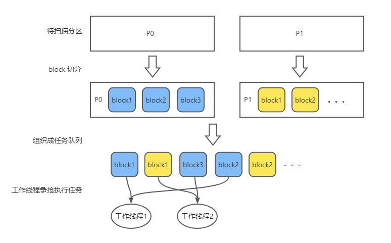
The optimizer automatically chooses whether to divide data into partition granules or block granules based on the specified degree of parallelism. If block granules are chosen, the parallel execution framework dynamically determines the block division at runtime to ensure that a block is neither too large nor too small. A block that is too large can cause data skew and lead to insufficient work for some threads. A block that is too small results in frequent switchovers for scans, causing high overheads.

Once the partition granularity (namely, the block granularity) is determined, a scan task corresponding to each granule is generated. The table scan operator sequentially processes these scan tasks and completes them one by one until all tasks are executed.

Producer-consumer pipeline model

Parallel execution is achieved by using the producer-consumer pipeline model.

After a parallel scheduling operator parses an execution plan, the plan is divided into multiple operation steps. Each operation step is called a DFO (Data Flow Operation).

Generally, the parallel scheduling operator starts two DFOS simultaneously. These two DFOS are connected in a producer-consumer manner to enable parallel execution between them. Each DFO uses a group of threads to execute tasks, which is called intra-DFO parallel execution. The number of threads used by an DFO is called the degree of parallelism (DOP).

In the next stage, the consumer DFO becomes the producer DFO. Under the coordination of the parallel scheduling operator, the consumer DFO and the producer DFO are started simultaneously. The following figure describes the flow of a DFO in the producer-consumer model.

• The data generated by DFO A is transmitted to DFO B for processing in real time.
• After DFO B completes the processing, the data is stored in the current thread and waits for the upstream DFO C to start.
• After receiving the start notification from DFO C, DFO B changes its role to a producer and begins to transmit data to DFO C. After receiving the data, DFO C starts to process the data.

In the following query example, the execution plan of the SELECT statement first scans the entire game table, then groups the data by team in the team table to calculate the sum of each group, and finally calculates the total scores of all teams.

CREATE TABLE game (round INT PRIMARY KEY, team VARCHAR(10), score INT)
     PARTITION BY HASH(round) PARTITIONS 3;
INSERT INTO game VALUES (1, "CN", 4), (2, "CN", 5), (3, "JP", 3);
INSERT INTO game VALUES (4, "CN", 4), (5, "US", 4), (6, "JP", 4);
SELECT /*+ PARALLEL(3) */ team, SUM(score) TOTAL FROM game GROUP BY team;

obclient> EXPLAIN SELECT /*+ PARALLEL(3) */ team, SUM(score) TOTAL FROM game GROUP BY team;
obclient> EXPLAIN SELECT /*+ PARALLEL(3) */ team, SUM(score) TOTAL FROM game GROUP BY team;
+---------------------------------------------------------------------------------------------------------+
| Query Plan                                                                                              |
+---------------------------------------------------------------------------------------------------------+
| =================================================================                                       |
| |ID|OPERATOR                     |NAME    |EST.ROWS|EST.TIME(us)|                                       |
| -----------------------------------------------------------------                                       |
| |0 |PX COORDINATOR               |        |1       |4           |                                       |
| |1 | EXCHANGE OUT DISTR          |:EX10001|1       |4           |                                       |
| |2 |  HASH GROUP BY              |        |1       |4           |                                       |
| |3 |   EXCHANGE IN DISTR         |        |3       |3           |                                       |
| |4 |    EXCHANGE OUT DISTR (HASH)|:EX10000|3       |3           |                                       |
| |5 |     HASH GROUP BY           |        |3       |2           |                                       |
| |6 |      PX BLOCK ITERATOR      |        |1       |2           |                                       |
| |7 |       TABLE SCAN            |game    |1       |2           |                                       |
| =================================================================                                       |
| Outputs & filters:                                                                                      |
| -------------------------------------                                                                   |
|   0 - output([INTERNAL_FUNCTION(game.team, T_FUN_SUM(T_FUN_SUM(game.score)))]), filter(nil), rowset=256 |
|   1 - output([INTERNAL_FUNCTION(game.team, T_FUN_SUM(T_FUN_SUM(game.score)))]), filter(nil), rowset=256 |
|       dop=3                                                                                             |
|   2 - output([game.team], [T_FUN_SUM(T_FUN_SUM(game.score))]), filter(nil), rowset=256                  |
|       group([game.team]), agg_func([T_FUN_SUM(T_FUN_SUM(game.score))])                                  |
|   3 - output([game.team], [T_FUN_SUM(game.score)]), filter(nil), rowset=256                             |
|   4 - output([game.team], [T_FUN_SUM(game.score)]), filter(nil), rowset=256                             |
|       (#keys=1, [game.team]), dop=3                                                                     |
|   5 - output([game.team], [T_FUN_SUM(game.score)]), filter(nil), rowset=256                             |
|       group([game.team]), agg_func([T_FUN_SUM(game.score)])                                             |
|   6 - output([game.team], [game.score]), filter(nil), rowset=256                                        |
|   7 - output([game.team], [game.score]), filter(nil), rowset=256                                        |
|       access([game.team], [game.score]), partitions(p[0-2])                                             |
|       is_index_back=false, is_global_index=false,                                                       |
|       range_key([game.round]), range(MIN ; MAX)always true                                              |
+---------------------------------------------------------------------------------------------------------+
29 rows in set

The following diagram shows the execution plan of the preceding query example:

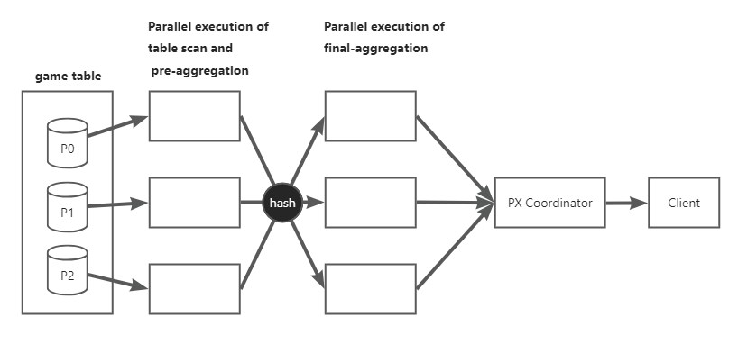
As shown in the figure, the query actually uses six threads. The execution flow and task distribution are as follows:

• Step 1: The first three threads scan the game table and pre-aggregate the game.team data within each thread.
• Step 2: The last three threads aggregate the pre-aggregated data.
• Step 3: The aggregated result is handed over to the parallel scheduling operator, which returns the result to the client.

When sending the data from Step 1 to Step 2, a hash join is used based on the game.team field to determine the destination thread for the pre-aggregated data.

Data distribution between producers and consumers

Data distribution refers to the method used to send data from a group of worker threads (producers) that execute in parallel to another group of worker threads (consumers). The optimizer selects the optimal data redistribution method to achieve the best performance by using a series of optimization strategies.

The following common data distribution methods are used in parallel execution:

• HASH DISTRIBUTION

  In HASH DISTRIBUTION, the producers hash and modulo the data rows based on the distribution key to determine the consumers to which they send the data. Generally, HASH DISTRIBUTION can distribute data evenly to multiple consumers.

• PKEY DISTRIBUTION

  In PKEY DISTRIBUTION, the producers calculate the partitions of the destination tables for the data rows and send the data rows to the consumers that process the partitions. PKEY DISTRIBUTION is commonly used in partial partition-wise join scenarios. In this scenario, the data on the consumer side does not need to be redistributed. Instead, the data can be partition-wise joined with the data on the producer side, reducing the network communication and enhancing the performance.

• PKEY HASH DISTRIBUTION

  In PKEY HASH DISTRIBUTION, the producers calculate the partitions of the destination tables for the data rows and then hash the data rows based on the distribution key to determine the consumers to which they send the data.

  PKEY HASH DISTRIBUTION is commonly used in parallel DML scenarios. In such scenarios, multiple threads can concurrently update data in one partition. Therefore, the PKEY HASH DISTRIBUTION method is used to ensure that data rows with the same value are processed by the same thread, and data rows with different values are distributed to multiple threads as evenly as possible.

• BROADCAST DISTRIBUTION

  In BROADCAST DISTRIBUTION, the producers send each data row to each consumer thread, ensuring that each consumer thread has all the data from the producers. Broadcast Distribution is commonly used to copy data of a small table to all nodes that execute the join operation and then perform the join operation by using the data on the local node to reduce the network communication.

• BC2HOST DISTRIBUTION

  In BC2HOST DISTRIBUTION, the producers send each data row to each consumer node, ensuring that each consumer node has all the data from the producers. Then, the consumer threads in the nodes work together to process the data.

  BC2HOST DISTRIBUTION is commonly used in NESTED LOOP JOIN and SHARED HASH JOIN scenarios. In the NESTED LOOP JOIN scenario, each consumer thread obtains a part of the shared data as the driving data and uses it to perform the join operation on the target table; in the SHARED HASH JOIN scenario, each consumer thread builds a hash table based on the shared data. This way, the data tables are jointly built by the threads without the need for each thread to build the same hash table, thus avoiding unnecessary overheads.

• RANGE DISTRIBUTION

  In RANGE DISTRIBUTION, the producers divide the data into segments based on ranges and distribute the data segments to the consumer threads so that each consumer thread handles data of a different range. RANGE DISTRIBUTION is commonly used in sorting scenarios. Each consumer thread needs to sort only the data it is allocated, to maintain the global order.

• RANDOM DISTRIBUTION

  In RANDOM DISTRIBUTION, the producers randomize the data and send the data to the consumer threads. This ensures that each consumer thread handles nearly the same amount of data, achieving load balancing. RANDOM DISTRIBUTION is commonly used in multi-threaded parallel UNION ALL scenarios. In such scenarios, it is necessary to disperse the data and achieve load balancing but not to maintain any other relationships among the data.

• HYBRID HASH DISTRIBUTION

  Hybrid HASH DISTRIBUTION is used in adaptive join algorithms. Based on the statistics collected, OceanBase Database provides a set of parameters to define regular values and frequent values. In the hybrid HASH DISTRIBUTION method, regular values on both sides of the join are distributed by using the HASH method, frequent values on the left side are distributed by using the BROADCAST method, and frequent values on the right side are distributed by using the RANDOM method.

  

Data transmission between producers and consumers

At any time, DFOs that are parallelly scheduled by the same operator are connected in a producer-consumer manner for parallel execution. To transmit data between producers and consumers, a data transmission network is needed to be created.

For example, if a data scan DFO uses DOP = 2 and a data aggregation DFO uses DOP = 3, each of the two producer threads creates three virtual links to connect to the consumer threads, resulting in a total of six virtual links. The following figure illustrates this scenario.

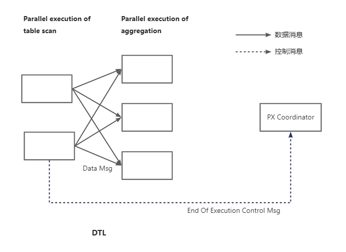
The virtual transmission network created is called the data transfer layer (DTL). In the parallel execution framework of OceanBase Database, all control messages and row data are transmitted through the DTL. Each worker thread can establish thousands of virtual links, demonstrating high scalability. Additionally, the DTL supports features such as data buffering, batch data transmission, and automatic flow control.

When the DTL is deployed on the same node, it uses memory copying to transmit messages; when the DTL is deployed on different nodes, it uses network communication to transmit messages.

Worker threads

In a parallel query, there are two types of threads: a main thread and multiple worker threads. The main thread runs in the thread pool that is also used for ordinary TP queries, whereas the worker threads run in a dedicated thread pool.

OceanBase Database uses a dedicated thread pool to allocate worker threads for parallel queries. Each tenant has a dedicated parallel execution thread pool on each node it belongs to. All worker threads for parallel queries are allocated from these thread pools.

Before a parallel scheduling operator schedules each DFO, it requests thread resources from the thread pool. After the DFO execution is completed, the thread resources are immediately released.

The initial size of the thread pool is 0, and it can grow dynamically based on the actual needs without an upper limit. To avoid excessive idle threads, the thread pool has an automatic thread recycling mechanism. For any thread:

• If it has been idle for more than 10 minutes and the thread pool still has more than 8 threads, the thread is recycled and destroyed.
• If it has been idle for more than 60 minutes, the thread is unconditionally destroyed.

Although the upper limit of the thread pool size is unlimited, two mechanisms generally set an upper limit to the actual thread pool size in most cases:

• Before parallel execution starts, you must reserve thread resources through the Admission module. You can only start execution after the reservation succeeds. This mechanism limits the number of concurrent queries. For more information, see Concurrency control and queuing.
• Each time when you request threads from the thread pool, the maximum number of threads that can be allocated to you at a time is N. Here, N is the result of the MIN_CPU of the tenant unit multiplied by the px_workers_per_cpu_quota tenant-level parameter. If the requested number of threads exceeds N, at most N threads will be allocated to you. The default value of px_workers_per_cpu_quota is 10. For example, the DOP of a DFO is 100. It needs to request 30 threads from node A and 70 threads from node B. If the MIN_CPU of the tenant unit is 4 and the px_workers_per_cpu_quota tenant-level parameter is 10, then N = 4 × 10 = 40. In this case, the DFO actually requests 30 threads from node A and 40 threads from node B. The actual DOP is 70.

Optimize performance by load balancing

To achieve the best performance, the tasks assigned to all worker threads should be as equal as possible.

When SQL uses a block granule to divide tasks, the system dynamically assigns tasks to worker threads. This approach minimizes workload imbalance, ensuring that no worker thread is obviously overloaded.

When SQL uses a partition granule to divide tasks, you can set the number of tasks to an integer multiple of the number of worker threads to optimize performance. This approach is useful in partition-wise join and parallel DML scenarios.

Assume that a table has 16 partitions with approximately equal data amounts. You can use 16 worker threads (with a DOP of 16) to complete the work in about 1/16 of the time; you can also use five worker threads (with a DOP of 5) to complete the work in about 1/5 of the time; or you can use two worker threads (with a DOP of 2) to complete the work in about half the time. However, if you use 15 worker threads to process 16 partitions, the first thread will start processing the 16th partition after it completes the first one. The other threads will become idle after they complete their work. If the data amounts in each partition are similar, this configuration results in poor performance. If the data amounts in each partition vary, the actual performance varies accordingly.

Likewise, assume that you use six worker threads to process 16 partitions with similar data amounts in each partition.

In this case, after each thread completes the work in the first partition, it will move on to the second partition. However, only four threads will process the third partition, and the other two threads will remain idle.

Generally, the time required to perform parallel operations on N partitions using P worker threads does not necessarily equal N divided by P. This formula does not take into account the fact that some threads may need to wait for other threads to complete the last partition. However, you can select an appropriate DOP to minimize workload imbalance and optimize performance.

Scenarios where parallel execution is not recommended

Parallel execution is not recommended in the following scenarios:

• Typical SQL queries in your system take milliseconds to complete.

  Parallel queries have scheduling overheads measured in milliseconds. For short queries, the scheduling overheads can offset the benefits of parallel execution.

• Your system is under high load.

  The design goal of parallel execution is to utilize idle system resources. If the system itself has no idle resources, parallel execution is unlikely to improve performance and may even degrade overall system performance.

Serial execution uses a single thread to perform database operations. Serial execution is preferable to parallel execution in the following scenarios:

• The query accesses a small amount of data.
• High concurrency is required.
• The query execution time is less than 100 ms.

Parallel execution cannot be enabled for the following scenarios:

• The top-level DFO does not require parallel execution. It is responsible for interactions with the client and performs operations that do not require parallel execution, such as LIMIT and PX COORDINATOR at the top level.
• A DFO containing a TABLE user-defined function (UDF) must be executed serially, but other DFOs can still be executed in parallel.
• Parallel execution is not supported for ordinary SELECT and DML statements in OLTP systems.