


An execution plan is a description of the process of executing an SQL query statement in a database.
You can use the EXPLAIN command to view the logical execution plan generated by the optimizer for a given SQL statement. To analyze performance issues of an SQL statement, you typically need to first view the SQL execution plan and check whether any issues exist at each step. Therefore, understanding the execution plan is a prerequisite for SQL tuning, and understanding the operators of an execution plan is key to understanding the EXPLAIN command.
Format of the EXPLAIN statement
OceanBase Database supports three EXPLAIN command formats: EXPLAIN BASIC, EXPLAIN, and EXPLAIN EXTENDED. These three formats display different levels of detail:
The
EXPLAIN BASICcommand shows the most basic plan display.The
EXPLAIN EXTENDEDcommand shows the most detailed plan display (usually used for troubleshooting).The
EXPLAINcommand shows information that helps users understand how the entire plan is executed.
The format of the EXPLAIN command is as follows:
EXPLAIN [BASIC | EXTENDED | PARTITIONS | FORMAT = format_name] [PRETTY | PRETTY_COLOR] explainable_stmt
format_name:
{ TRADITIONAL | JSON }
explainable_stmt:
{ SELECT statement
| DELETE statement
| INSERT statement
| REPLACE statement
| UPDATE statement }
The EXPLAIN command applies to SELECT, DELETE, INSERT, REPLACE, and UPDATE statements. It displays information about the statement execution plan provided by the optimizer, including how the statement is processed, how tables are joined, and the join order.
Generally, you can use the EXPLAIN EXTENDED command to display the scan range of the table. You can use the EXPLAIN OUTLINE command to display the outline information.
The FORMAT option is used to select the output format. TRADITIONAL displays output in table format, which is the default. JSON displays information in JSON format.
You can use EXPLAIN PARTITIONS to check queries involving partitioned tables. If you check queries for non-partitioned tables, no error is returned, but the values in the PARTITIONS column are always NULL.
For complex execution plans, you can use the PRETTY or PRETTY_COLOR option to connect the parent and child nodes in the plan tree with tree lines or colored tree lines, so that the execution plan is easier to read. Here is an example:
obclient> CREATE TABLE p1table(c1 INT ,c2 INT) PARTITION BY HASH(c1) PARTITIONS 2;
Query OK, 0 rows affected
obclient> CREATE TABLE p2table(c1 INT ,c2 INT) PARTITION BY HASH(c1) PARTITIONS 4;
Query OK, 0 rows affected
obclient> EXPLAIN EXTENDED PRETTY_COLOR SELECT * FROM p1table p1 JOIN p2table p2 ON p1.c1=p2.c2\G
*************************** 1. row ***************************
Query Plan: ==========================================================
|ID|OPERATOR |NAME |EST. ROWS|COST|
----------------------------------------------------------
|0 |PX COORDINATOR | |1 |278 |
|1 | EXCHANGE OUT DISTR |:EX10001|1 |277 |
|2 | HASH JOIN | |1 |276 |
|3 | ├PX PARTITION ITERATOR | |1 |92 |
|4 | │ TABLE SCAN |P1 |1 |92 |
|5 | └EXCHANGE IN DISTR | |1 |184 |
|6 | EXCHANGE OUT DISTR (PKEY)|:EX10000|1 |184 |
|7 | PX PARTITION ITERATOR | |1 |183 |
|8 | TABLE SCAN |P2 |1 |183 |
==========================================================
Outputs & filters:
-------------------------------------
0 - output([INTERNAL_FUNCTION(P1.C1, P1.C2, P2.C1, P2.C2)]), filter(nil)
1 - output([INTERNAL_FUNCTION(P1.C1, P1.C2, P2.C1, P2.C2)]), filter(nil), dop=1
2 - output([P1.C1], [P2.C2], [P1.C2], [P2.C1]), filter(nil),
equal_conds([P1.C1 = P2.C2]), other_conds(nil)
3 - output([P1.C1], [P1.C2]), filter(nil)
4 - output([P1.C1], [P1.C2]), filter(nil),
access([P1.C1], [P1.C2]), partitions(p[0-1])
5 - output([P2.C2], [P2.C1]), filter(nil)
6 - (#keys=1, [P2.C2]), output([P2.C2], [P2.C1]), filter(nil), dop=1
7 - output([P2.C1], [P2.C2]), filter(nil)
8 - output([P2.C1], [P2.C2]), filter(nil),
access([P2.C1], [P2.C2]), partitions(p[0-3])
1 row in set
Shape and operators of a plan
A sample execution plan in OceanBase Database is as follows:
|ID|OPERATOR |NAME |EST. ROWS|COST |
-------------------------------------------------------
|0 |LIMIT | |100 |81141|
|1 | TOP-N SORT | |100 |81127|
|2 | HASH GROUP BY | |2924 |68551|
|3 | HASH JOIN | |2924 |65004|
|4 | SUBPLAN SCAN |VIEW1 |2953 |19070|
|5 | HASH GROUP BY | |2953 |18662|
|6 | NESTED-LOOP JOIN| |2953 |15080|
|7 | TABLE SCAN |ITEM |19 |11841|
|8 | TABLE SCAN |STORE_SALES|161 |73 |
|9 | TABLE SCAN |DT |6088 |29401|
=======================================================
You may notice from the foregoing examples that a plan in OceanBase Database is similar to that in Oracle Database. The following table describes columns of an execution plan in OceanBase Database.
Column |
Description |
|---|---|
| ID | The sequence number of the execution tree obtained by using preorder traversal, starting from 0. |
| OPERATOR | The name of the operator. |
| NAME | The name of the table or index corresponding to a table operation. |
| EST. ROWS | The estimated number of output rows of the operator. |
| COST | The execution cost of the operator, in microseconds. |
Note
In a table operation, the NAME field displays names (alias) of tables involved in the operation. In the case of index access, the name of the index is displayed in parentheses after the table name. For example, t1(t1_c2) indicates that index t1_c2 is used. In the case of reverse scanning, the keyword RESERVE is added after the index name, with the index name and the keyword RESERVE separated with a comma (,), such as t1(t1_c2,RESERVE).
In OceanBase Database, the first part of the output of the EXPLAIN command is the tree structure of the execution plan. The hierarchy of operations in the tree is represented by the indentation of the operators. Operators at the deepest level are executed first. Operators at the same level are executed in the specified execution order.
The following figure shows the tree structure of the execution plan described in the preceding example:
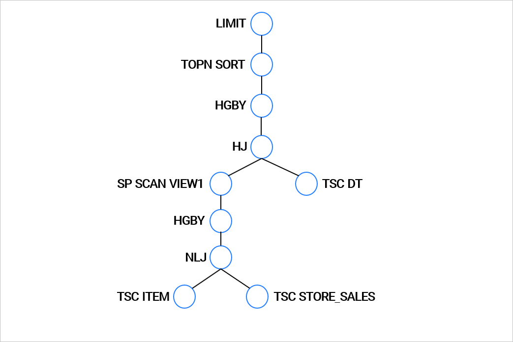
In OceanBase Database, the second part of the output of the EXPLAIN command contains the details of each operator, including the output expression, filter conditions, partition information, and unique information of each operator, such as the sort keys, join keys, and pushdown conditions. Here is an example:
Outputs & filters:
-------------------------------------
0 - output([t1.c1], [t1.c2], [t2.c1], [t2.c2]), filter(nil), sort_keys([t1.c1, ASC], [t1.c2, ASC]), prefix_pos(1)
1 - output([t1.c1], [t1.c2], [t2.c1], [t2.c2]), filter(nil),
equal_conds([t1.c1 = t2.c2]), other_conds(nil)
2 - output([t2.c1], [t2.c2]), filter(nil), sort_keys([t2.c2, ASC])
3 - output([t2.c2], [t2.c1]), filter(nil),
access([t2.c2], [t2.c1]), partitions(p0)
4 - output([t1.c1], [t1.c2]), filter(nil),
access([t1.c1], [t1.c2]), partitions(p0)