Table overview

In OceanBase Database, a table is the basic unit of data storage. A table contains all the data that users can access. Each table consists of multiple rows, and each row contains multiple columns. The design and usage of each table must be reasonably planned based on business requirements to ensure the system's efficiency and scalability.

Table types

OceanBase Database supports various table types, including partitioned tables, replicated tables, primary key tables, non-primary key tables, and external tables.

• Partitioned tables: OceanBase Database divides the data of a regular table into different partitions based on specific rules and stores the data of the same partition together. This type of table is called a partitioned table. OceanBase Database supports basic partitioning strategies, including range partitioning, list partitioning, and hash partitioning.
• Replicated tables: Replicated tables are a special type of table in OceanBase Database. Data in these tables can be read from any "healthy" replica.
• Primary key tables and non-primary key tables: A primary key table is a table that contains a primary key. A non-primary key table is a table that does not specify a primary key.
• External tables: The data of a regular table is stored in the storage space of the database, while the data of an external table is stored in an external storage service.
• Heap tables: In a heap-organized table, the primary key is used to enforce uniqueness, and queries rely on the primary table. When user data is sorted by time, the Skip Index feature can be used to improve query efficiency.

In AP scenarios, OceanBase Database supports various table types, including replicated tables, partitioned tables, primary key tables, and non-primary key tables, which are commonly used in TP scenarios. Based on the data storage method, which is row-based or column-based, new table types have been introduced: columnstore tables and hybrid row-columnstore tables.

• Columnstore tables: Columnstore tables store data by column rather than by row, which significantly improves the performance of analytical queries, especially for large datasets and frequent aggregation analysis. For more information, see Columnstore tables.

• Hybrid row-columnstore tables: These tables store both row-based and column-based data. The system automatically determines whether to use row-based or column-based queries based on the query statement, making them suitable for scenarios that require both transactional and analytical operations.

Table update modes

OceanBase Database allows you to specify the write and query modes when creating a table. When creating a table, you can use the merge_engine parameter in the CREATE TABLE statement to choose between delete_insert update mode and partial_update update mode. These two modes are data update strategies designed for different business scenarios.

• delete_insert (full-column update mode)

  This mode prioritizes query performance. It uses the "Merge-On-Write" mechanism to convert UPDATE operations into full-column DELETE and INSERT records, ensuring that each row contains complete column values. This mode significantly improves the efficiency of complex queries and batch processing (such as analytical tasks), but it requires additional storage space for incremental data. It is suitable for scenarios with frequent incremental data and the need for quick analysis.

• partial_update (partial update mode)

  This mode only records the values of modified columns, avoiding redundant storage. During queries, multiple data sets need to be merged to obtain the latest values, which results in relatively lower performance. However, it is more suitable for scenarios with frequent updates but low query requirements (such as OLTP operations) or environments where storage costs are a concern.

For more information, see Create a table in MySQL-compatible mode and Create a table in Oracle-compatible mode.

Data distribution

OceanBase Database distributes data across different partitions by creating partitioned tables. Data in different partitions can be distributed across different machines. During queries, partition pruning reduces the amount of data scanned and leverages multi-machine resources to enhance query performance. By default, data between different tables is randomly distributed and has no direct relationship. Load balancing ensures that data from a table is evenly distributed across the entire cluster.

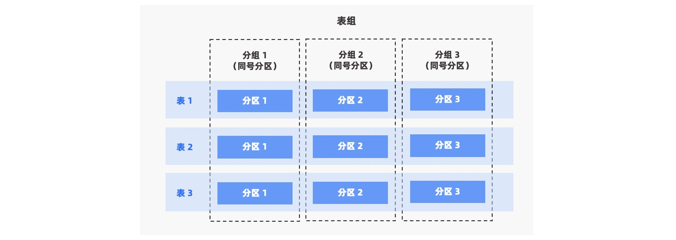
In a distributed AP system, tables often contain a large amount of data. When data from different tables is randomly distributed, the overhead of data transmission during table joins can be significant. Using table groups (Table Group) allows partitioned tables with the same partitioning strategy to align data according to specific rules. This aggregates related data on the same machine, enabling the use of Partition Wise Join during table joins, which effectively reduces data transmission overhead and improves performance.

OceanBase Database supports both primary and secondary partitioned tables and provides three types of partitioning: RANGE, LIST, and HASH.

OceanBase Database provides three types of table groups:

1. NONE: All tables in the table group are aggregated on the same machine.

2. PARTITION: Data of each table in the table group is scattered by primary partitions. For secondary partitioned tables, all secondary partitions under each primary partition are aggregated together.

3. ADAPTIVE: Data of each table in the table group is scattered adaptively. For primary partitioned tables, data is scattered by primary partitions; for secondary partitioned tables, data is scattered by secondary partitions under each primary partition.

For more information, see Data distribution, Table groups in MySQL-compatible mode, and Table groups in Oracle-compatible mode.

Index types

Indexes are key components for improving query performance. OceanBase Database provides flexible and efficient data retrieval methods in AP scenarios by supporting various index types. The following are some common index types and their application scenarios:

• Local indexes: Local indexes are indexes created for a single partition. They are suitable for scenarios requiring local data queries. When data is strictly partitioned, local indexes can significantly reduce the data scanning scope during queries, thereby improving query efficiency.
• Unique indexes: Unique indexes ensure that each value in the indexed column is unique. By creating unique indexes on certain columns, databases can effectively prevent data duplication and accelerate query processes.
• Non-unique indexes: Unlike unique indexes, non-unique indexes do not require all values in the indexed column to be unique. They are primarily used to accelerate data queries, especially when searching for multiple records that meet specific conditions.
• Full-text indexes: OceanBase Database supports full-text search capabilities compatible with MySQL. By preprocessing text content and creating keyword indexes, full-text search efficiency is significantly improved. For more information about full-text indexes, see Full-text indexes.
• JSON multi-value indexes: OceanBase Database's MySQL-compatible mode supports multi-value indexes, which are particularly useful for JSON documents and other collection data types. This feature allows indexes to be created on arrays or collections, enhancing query efficiency when searching for JSON array elements. For more information about multi-value indexes, see Multi-value indexes.
• Spatial indexes: Spatial indexes optimize the query efficiency of geographic space data and are widely used in geographic information systems (GIS) and location-based services. In these applications, spatial indexes can quickly retrieve data within a geographic coordinate range, providing strong support for location services.
• Columnstore indexes: In HTAP (Hybrid Transactional and Analytical Processing) scenarios, OceanBase Database supports creating tables with columnar storage format starting from version V4.3.0. Indexes and data tables are both tables, so columnar storage can also be set for index tables. Columnstore indexes store data based on columns rather than rows, significantly improving the performance of analytical queries, especially when handling large-scale data, by greatly reducing the time required for data retrieval and analysis. For more information about columnar storage, see Columnar storage.

For more information about indexes, see Overview of indexes in MySQL-compatible mode and Overview of indexes in Oracle-compatible mode.

Data types

Before creating and using tables, database administrators need to plan the table structure and data types based on business requirements. To ensure efficient data storage and query optimization, administrators should follow these principles:

• Normalize the table structure: Design the table structure reasonably to minimize data redundancy and improve query efficiency.
• Choose appropriate SQL data types: Select the most suitable SQL data type for each column to reduce storage space and enhance query speed.

Common SQL data types include:

• Basic data types: such as INT, VARCHAR, and DATE.
• Complex data types: such as JSON, ARRAY, and BITMAP, suitable for storing more complex data structures.

For detailed descriptions of SQL data types, see:

• Data types in MySQL-compatible mode
• Data types in Oracle-compatible mode

Views

OceanBase Database supports standard views and materialized views.

• Standard views: Standard views, also known as non-materialized views, are the most common type of view. They store only the SQL query that defines the view, not the query results.
• Materialized views: Unlike standard views, materialized views store the query results physically. OceanBase Database supports asynchronous materialized views, where the materialized view is not immediately updated when the base table data changes, ensuring the execution performance of DML operations on the base table. For more information, see Materialized views in MySQL-compatible mode and Materialized views in Oracle-compatible mode.

Example of creating a data table

Create a table that includes partitions, columnstore, and rowstore indexes.

CREATE TABLE salesdata (
    sale_id INT,
    product_id INT NOT NULL,
    saledate DATE NOT NULL,
    saledate_int INT, -- Defined as a regular column
    quantity INT,
    price DECIMAL(10, 2),
    customer_id INT,
    PRIMARY KEY (sale_id, saledate_int) -- The primary key can include regular columns
)
PARTITION BY RANGE COLUMNS (saledate_int) (
    PARTITION p2023_q1 VALUES LESS THAN (202304),
    PARTITION p2023_q2 VALUES LESS THAN (202307),
    PARTITION p2023_q3 VALUES LESS THAN (202310),
    PARTITION p2023_q4 VALUES LESS THAN (202401)
)
WITH COLUMN GROUP(each column);

CREATE INDEX idx_product_id ON salesdata(product_id);
CREATE INDEX idx_customer_id ON salesdata(customer_id);

1. Partitioning: The salesdata table uses range partitioning (RANGE).

   • PARTITION BY RANGE COLUMNS (saledate_int): Partitions the table by the saledate_int column.

   • Four partitions are defined:

     • The p2023_q1 partition contains data before 202304 (i.e., data from the first quarter of 2023).
     • The p2023_q2, p2023_q3, and p2023_q4 partitions contain data from the second, third, and fourth quarters of 2023, respectively.

2. Columnstore: Columnstore storage is specified using WITH COLUMN GROUP(each column);. Data in these columns will be stored in a columnar format, making it suitable for large-scale data analysis.

3. Rowstore indexes: Two rowstore indexes, idx_product_id and idx_customer_id, are created on the product_id and customer_id columns, respectively. Rowstore indexes can accelerate queries that target specific columns, especially for high-frequency small queries.

When creating and using a columnstore table, if you import a large amount of data, note that you must perform a major compaction to improve read performance and collect statistics to adjust the execution strategy.

• Major compaction: After you import data in batches, we recommend that you perform a major compaction. This improves read performance because the compaction operation compacts fragmented data to make it more contiguous in physical storage, thereby reducing the disk I/O required for read operations. After you import data, trigger a major compaction in the tenant to ensure that all data is compacted to the baseline layer. For more information, see MAJOR and MINOR (MySQL-compatible mode) and MAJOR and MINOR (Oracle-compatible mode).

• Collect statistics: After the major compaction is completed, we recommend that you collect statistics. This is important for the optimizer to generate effective query plans and execution strategies. For more information, see GATHER_SCHEMA_STATS (MySQL-compatible mode) and GATHER_SCHEMA_STATS (Oracle-compatible mode). You can also use the views GV$OB_OPT_STAT_GATHER_MONITOR (MySQL-compatible mode) and GV$OB_OPT_STAT_GATHER_MONITOR (Oracle-compatible mode) to monitor the collection progress.

Note that as the amount of data in columnstore tables increases, the speed of major compaction may decrease.