







In OceanBase Database V3.x, replicas are distributed across multiple nodes on a per-partition basis. The load balancing module can achieve intra-tenant partition balancing through methods such as partition leader switchover and partition replica migration. After upgrading to the standalone log stream architecture in V4.x, replicas are distributed on a per-log stream basis, with each log stream carrying a large number of partitions. Therefore, in V4.2.x, the load balancing module cannot directly control partition distribution. Instead, it must first balance the number of LSs (Log Streams) and leaders, and then perform partition balancing based on the log stream distribution.
Notice
Partition balancing applies only to user tables.
The priority order for LS balancing and partition balancing is as follows:
LS balancing > Partition balancing
Load balancing of leaders (Homogeneous zone mode)
Load balancing of leaders
When you perform operations such as changing the number of units (UNIT_NUM) for a tenant, modifying the first priority of the PRIMARY_ZONE, or modifying the locality (which affects the PRIMARY_ZONE), the background threads of the load balancing module immediately adjust the number and location of leaders by splitting, merging, or reassigning leader groups to match the modified tenant state. Specifically, each tenant's units are assigned to a log stream group, where the number of log streams equals the number of zones in the first-priority zone of the PRIMARY_ZONE. Leaders are then evenly distributed across zones within these log stream groups.
Note
- A log stream group is an attribute of a leader. Log streams with the same log stream group ID are aggregated together.
- In homogeneous zone mode of V4.x, OceanBase Database requires that the number of units per zone within a tenant must be consistent. To facilitate unified management of units across zones, the system introduces the unit group mechanism. Units with the same unit group ID belong to the same unit group. All units within a unit group have identical data distributions, the same log stream replicas, and serve the same partition data. From a resource container perspective, a unit group defines a set of data, which is served by one or more log streams, and read/write service capabilities can be scaled out to multiple units within the unit group.
- In homogeneous zone mode, a log stream group uniquely corresponds to a unit group. That is, log streams with the same log stream group ID are distributed within the same unit group.
In homogeneous zone mode, the formula for calculating the number of leaders is as follows:
Number of leaders = UNIT_NUM * first_level_primary_zone_num
Note
The number of leaders here refers to user log streams, excluding system log streams and broadcast log streams.
The following table describes scenarios for load balancing of leaders.
Examples of scenarios triggering load balancing |
Balancing Condition |
Balancing algorithm |
LS Balancing Strategy |
|---|---|---|---|
PRIMARY_ZONE: Fromz1, z2Changed toz1Also, UNIT_NUM: From1Changed to2 |
Some LS groups have missing LSs, while others have extra LSs, but the total number of LSs matches the final state. | Migrate redundant LS to the LS Group lacking LS | LS_BALANCE_BY_MIGRATE |
PRIMARY_ZONE: Fromz1Changed toz1,z2or UNIT_NUM: From2Changed to3 |
Only LS Group is missing LS | Assume the number of LSs is M before expansion and N after expansion (M < N). Each missing LS requires a new LS to be created.M/NTablets |
LS_BALANCE_BY_EXPAND |
PRIMARY_ZONE: Fromz1,z2Changed toz1or UNIT_NUM: From3Changed to2 |
Only the LS Group has excess LS | Assume the current number of load servers is M, and you need to scale down to N load servers (M > N). Then each of the remaining load servers needs to handle a share of the traffic equal to(M-N)/NTablets |
LS_BALANCE_BY_SHRINK |
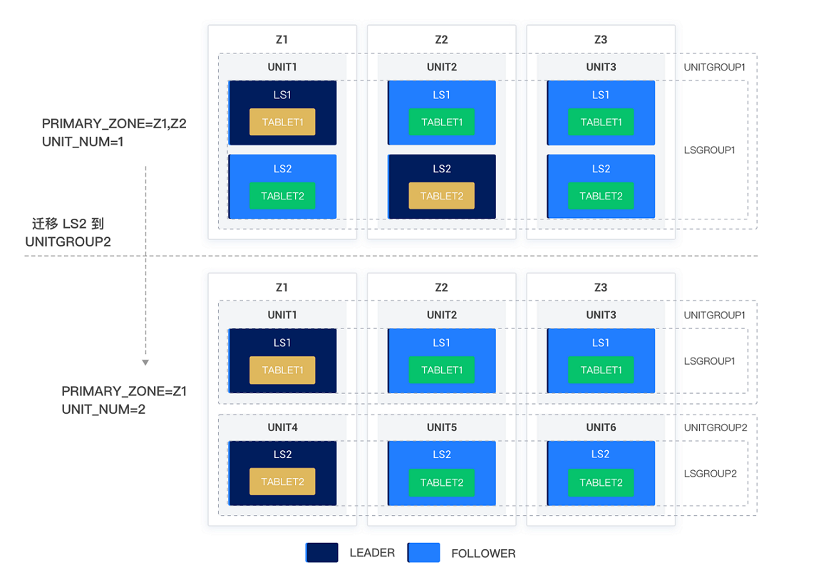
Example 1: As shown in the following figure, the first priority of the PRIMARY_ZONE changes from Z1, Z2 to Z1, and the UNIT_NUM changes from 1 to 2. Before and after the change, the number of leaders remains unchanged. The system directly migrates LS2 to the new unit. LS2 switches its leader to Z1 according to the change in PRIMARY_ZONE, thereby completing load balancing.
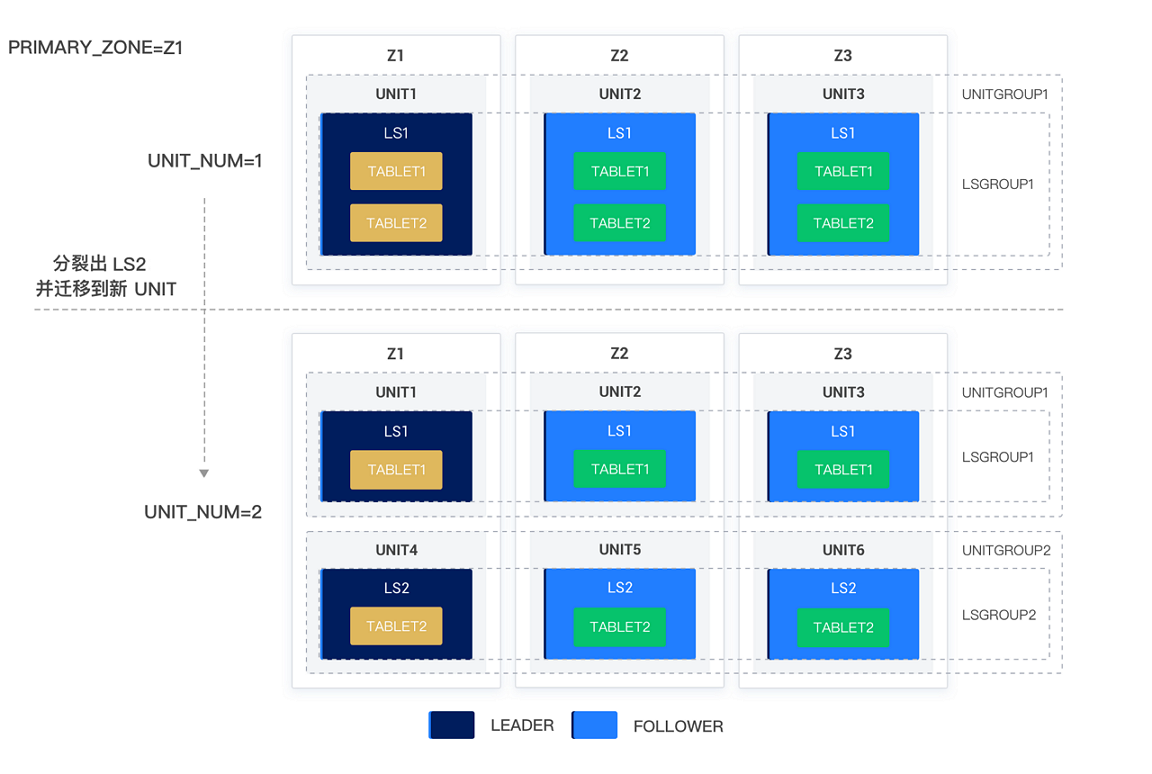
Example 2: As shown in the following figure, PRIMARY_ZONE = Z1, and UNIT_NUM changes from 1 to 2. To ensure there is a leader for each unit, LS2 is split to take away half of the tablets and migrate them to the new unit.
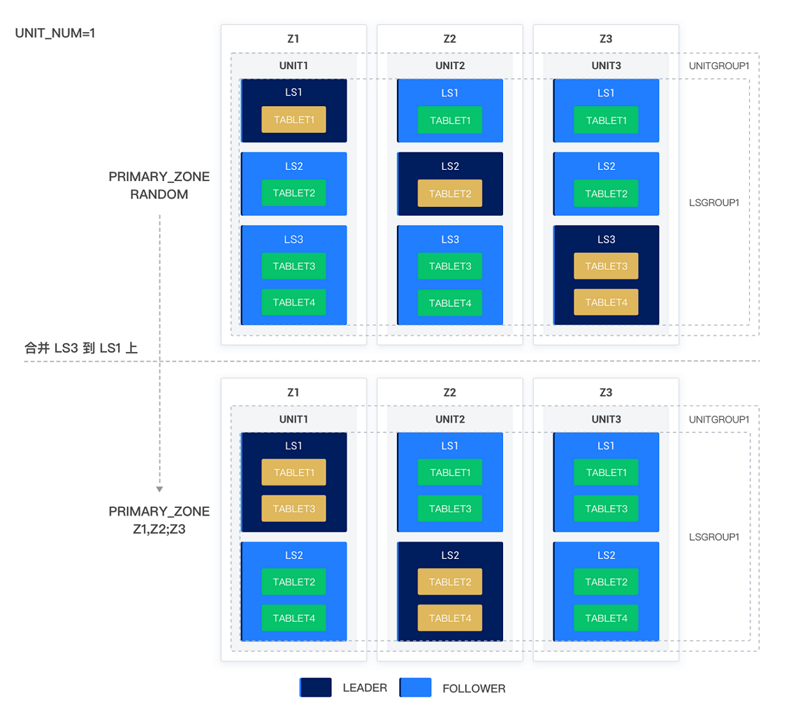
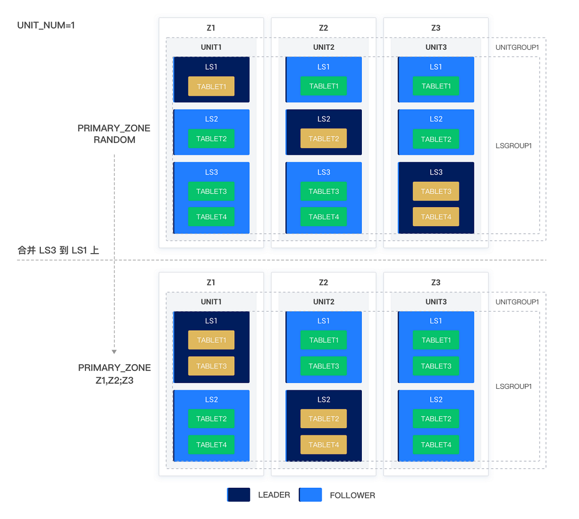
Example 3: As shown in the following figure, UNIT_NUM = 1, and the first priority of the PRIMARY_ZONE changes from RANDOM to Z1,Z2. To ensure leaders reside only on zones of the PRIMARY_ZONE with the highest priority and to maintain balanced tablet counts across log streams after balancing, since LS3 is in the same log stream group as the other leaders, half of the tablets from LS3 can be transferred to LS1. Then, LS3 can be merged into LS2, allowing LS2 to handle the remaining half of the tablets. This reduces the number of leaders while maintaining balanced tablet counts.
Load balancing of leaders across zones
Load balancing of leaders across zones ensures that leaders are evenly distributed across primary zones, given that the number of leaders is balanced. For example, after you change the PRIMARY_ZONE of a tenant, the background threads of the load balancing module dynamically adjust the number of leaders based on the first priority of the PRIMARY_ZONE and then perform leader switchover for the leaders to ensure that each zone in the first-priority zone has exactly one leader.
Automatic leader balancing is controlled by the tenant-level parameter enable_ls_leader_balance and is enabled by default.
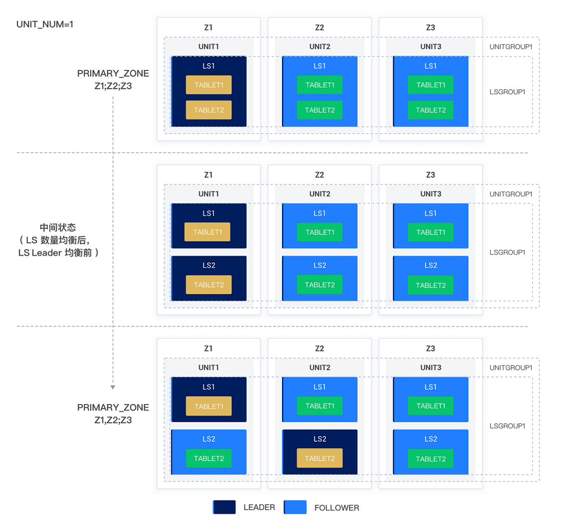
Example 1: As shown in the following figure, UNIT_NUM = 1, and the first priority of the PRIMARY_ZONE changes from Z1 to Z1,Z2. To ensure there is a leader in all zones of the first-priority zone, a new leader is split from the same unit, and then the leader of the new leader is switched to Z2 through leader balancing.
Example 2: As shown in the following figure, when UNIT_NUM = 1 and the first priority of PRIMARY_ZONE changes from RANDOM to Z1,Z2, after balancing the number of leaders by merging LS3 into other leaders, the remaining leader leaders are naturally and evenly distributed across Z1 and Z2. No additional leader leader balancing is required.
Load balancing in heterogeneous zones
In the current version, OceanBase Database also supports the heterogeneous zone mode for tenants. In heterogeneous zone mode, the number of units in each zone of a tenant can be different, but a tenant is limited to at most two UNIT_NUM values.
In heterogeneous zone mode, the load balancing algorithm controls the distribution of log streams at the granularity of units:
Within each zone of a tenant, the number of log streams per unit is equal.
Log streams are aggregated in a homogeneous manner within zones with the same
UNIT_NUM.
In heterogeneous zone mode, the formula for calculating the number of load balancing instances is as follows:
Number of load balancing instances = (Least Common Multiple of all UNIT_NUM values of the tenant) * first_level_primary_zone_num
Partition allocation during table creation
When you create a user table, OceanBase Database applies a balancing distribution strategy to scatter or aggregate partitions across various user log streams, ensuring a relatively balanced distribution of partitions on each stream.
User tables of specified table groups
You can specify a table group to flexibly configure the aggregation and sharding rules between different tables. When creating a user table, if you specify a table group for its Sharding and SCOPE attributes, the partitions of the new user table will be allocated to the corresponding user's LS according to the table group's rules. The table group rules are shown in the following table.
SHARDING / SCOPE attribute value |
SERVER |
ZONE |
CLUSTER |
|---|---|---|---|
| NONE | All partitions within the table group are aggregated on the same node (the partition distribution method is equivalent to SHARDING = NONE in earlier versions). |
All partitions within the table group are evenly distributed across zones. | All partitions within the table group are evenly distributed across all nodes. |
| PARTITION | Not supported | Not supported | Aggregated by primary partition, then randomly distributed among partition groups. (The partition distribution method is equivalent to SHARDING = PARTITION in earlier versions.) |
| SUBPARTITION | Not supported | Not supported | Aggregated by secondary partition, then distributed across the entire cluster for each partition group. |
| ADAPTIVE | Not supported | Not supported |
The partition distribution method is equivalent to |
Notice
If a user table already exists in the table group before you create a new table, the new table will be aligned with the partition distribution of the user table having the smallest table_id in the table group.
For more information about table groups, see About table groups.
Normal user tables
When creating a regular user table without specifying a Table Group, OceanBase Database disperses the new partitions across all user LSs by default. The specific rules are as follows.
Non-partitioned tables: A new partition is created and allocated to the user LS with the fewest partitions.
Partitioned tables: In a partitioned table, data is evenly distributed across all user LSs using the round-robin algorithm.
Subpartitioned tables: In a subpartitioned table, all subpartitions within each partition are evenly distributed across all user LSs using the round-robin algorithm.
The following examples illustrate this point.
Example 1: In MySQL-compatible mode, four non-partitioned tables named
tt1,tt2,tt3, andtt4are created.obclient [test]> CREATE TABLE tt1(c1 int);obclient [test]> CREATE TABLE tt2(c1 int);obclient [test]> CREATE TABLE tt3(c1 int);obclient [test]> CREATE TABLE tt4(c1 int);Query the partition distribution of four tables.
obclient [test]> SELECT table_name,partition_name,subpartition_name,ls_id,zone FROM oceanbase.DBA_OB_TABLE_LOCATIONS WHERE table_name in('tt1','tt2','tt3','tt4') AND role='LEADER';The query result is as follows.
+------------+----------------+-------------------+-------+------+ | table_name | partition_name | subpartition_name | ls_id | zone | +------------+----------------+-------------------+-------+------+ | tt1 | NULL | NULL | 1001 | z1 | | tt2 | NULL | NULL | 1002 | z2 | | tt3 | NULL | NULL | 1003 | z3 | | tt4 | NULL | NULL | 1001 | z1 | +------------+----------------+-------------------+-------+------+ 4 rows in setExample 2: Create another partitioned table named
tt5.obclient [test]> CREATE TABLE tt5(c1 int) PARTITION BY HASH(c1) PARTITIONS 6;View the distribution of this partitioned table.
obclient [test]> SELECT table_name,partition_name,subpartition_name,ls_id,zone FROM oceanbase.DBA_OB_TABLE_LOCATIONS WHERE table_name ='tt5' AND role='LEADER';The query result is as follows. The partitions of this table are evenly distributed across log streams such as
1001,1002, and1003using the round-robin algorithm.+------------+----------------+-------------------+-------+------+ | table_name | partition_name | subpartition_name | ls_id | zone | +------------+----------------+-------------------+-------+------+ | tt5 | p0 | NULL | 1003 | z3 | | tt5 | p1 | NULL | 1001 | z1 | | tt5 | p2 | NULL | 1002 | z2 | | tt5 | p3 | NULL | 1003 | z3 | | tt5 | p4 | NULL | 1001 | z1 | | tt5 | p5 | NULL | 1002 | z2 | +------------+----------------+-------------------+-------+------+ 6 rows in setExample 3: Create a subpartitioned table named
tt8.obclient [test]> CREATE TABLE tt8 (c1 int, c2 int, PRIMARY KEY(c1, c2)) PARTITION BY HASH(c1) SUBPARTITION BY RANGE(c2) SUBPARTITION TEMPLATE (SUBPARTITION p0 VALUES LESS THAN (1990), SUBPARTITION p1 VALUES LESS THAN (2000), SUBPARTITION p2 VALUES LESS THAN (3000), SUBPARTITION p3 VALUES LESS THAN (4000), SUBPARTITION p4 VALUES LESS THAN (5000), SUBPARTITION p5 VALUES LESS THAN (MAXVALUE)) PARTITIONS 2;View the partition distribution of the
tt8table.obclient [test]> SELECT table_name,partition_name,subpartition_name,ls_id,zone FROM oceanbase.DBA_OB_TABLE_LOCATIONS WHERE table_name ='tt8' AND role='LEADER';The query result is as follows. All subpartitions of the next-level partitions in this table are evenly distributed across all user LSs using the round-robin algorithm.
+------------+----------------+-------------------+-------+------+ | table_name | partition_name | subpartition_name | ls_id | zone | +------------+----------------+-------------------+-------+------+ | tt8 | p0 | p0sp0 | 1001 | z1 | | tt8 | p0 | p0sp1 | 1002 | z2 | | tt8 | p0 | p0sp2 | 1003 | z3 | | tt8 | p0 | p0sp3 | 1001 | z1 | | tt8 | p0 | p0sp4 | 1002 | z2 | | tt8 | p0 | p0sp5 | 1003 | z3 | | tt8 | p1 | p1sp0 | 1002 | z2 | | tt8 | p1 | p1sp1 | 1003 | z3 | | tt8 | p1 | p1sp2 | 1001 | z1 | | tt8 | p1 | p1sp3 | 1002 | z2 | | tt8 | p1 | p1sp4 | 1003 | z3 | | tt8 | p1 | p1sp5 | 1001 | z1 | +------------+----------------+-------------------+-------+------+ 12 rows in set
Special user tables
In addition to regular user tables, there are special user tables such as local index tables, global index tables, and replication tables, which have specific allocation rules. The details are as follows:
Local index table: It follows the same partitioning rule as the primary table. Each partition is bound to the partition distribution of the primary table.
Global index table: By default, it is a non-partitioned table. When created, it is distributed to the user LS with the fewest partitions.
Replication table: Replication tables exist only on broadcast log streams.
Partition balancing
Based on load balancing, the load balancing module disperses or aggregates partition tablets across different load servers through transfer to achieve balanced partitions for a tenant. The partition balancing task SCHEDULED_TRIGGER_PARTITION_BALANCE is controlled by the DBMS_BALANCE.TRIGGER_PARTITION_BALANCE subprogram and triggers partition balancing at 00:00 every day by default. For more information about partition balancing, see Configure scheduled partition balancing tasks.
The priority order of partition balancing strategies is as follows:
Partition attribute alignment > Table group and partition weight balancing > Number of partitions balancing > Partition disk balancing
Partition attribute alignment
Table group alignment
When you modify the table group attribute, SHARDING attribute, or SCOPE attribute of a table using an SQL statement, you must wait for the background partition balancing task to complete to achieve the desired partition distribution. You can manually trigger a partition balancing by calling the DBMS_BALANCE.TRIGGER_PARTITION_BALANCE subprogram to quickly align the attributes.
For the partition distribution rules of tables within a table group, see the User tables with specified table groups section in this topic.
For more information about table groups, see About table groups.
Duplicate_scope alignment
In the current version of OceanBase Database, changes to the attributes of a replicated table are supported. A replicated table can only exist on a broadcast log stream. After you modify the duplicate_scope attribute, you must wait for the partition balancing to complete before the table can be used with the expected attributes. You can manually trigger a partition balancing by calling the DBMS_BALANCE.TRIGGER_PARTITION_BALANCE subprogram to quickly align the attributes.
For detailed operations on changing the attributes of a replicated table, see Change the attributes of a replicated table (MySQL-compatible mode) and Change the attributes of a replicated table (Oracle-compatible mode).
Table group and partition weight balancing
Table group weight balancing
In the MySQL-compatible mode of OceanBase Database, user tables are aggregated by binding a database to a table group with SHARDING = 'NONE'. Currently, automatic aggregation of user tables within a single database and aggregation of user tables across multiple databases is supported.
You can achieve table group weight balancing by setting weights for a table group with SHARDING = 'NONE', so that the tables within the group are distributed according to their weights.
Table group weight balancing is a process within the PARTITION_BALANCE task. It can be triggered manually by the user tenant or automatically by a scheduled partition balancing task.
Partition weight balancing (non-table group)
Partition weight is the relative proportion of resources such as CPU, memory, and disk allocated among partitions set by the user. Only integer values are supported, with a range of [1, +∞). By default, a partition has no weight.
Non-table group partition weight balancing is a process within the PARTITION_BALANCE task. After you set partition weights for tables, you can trigger a partition balancing task manually or wait for a scheduled task to do so. The partition weight balancing algorithm minimizes the variance of the sum of partition weights across user log streams through partition movement and exchange.
Only tables with assigned partition weights participate in partition weight balancing. For partitions in a table without assigned weights, balancing is performed based on the number of partitions.
Applications of partition weight balancing
Non-table group partition weights are primarily used to distribute partition hotspots, supporting the following two scenarios:
Distribute hotspots within a partitioned table
Distribute hotspots between non-partitioned tables
Note
- Balancing within a subpartitioned table is not currently supported.
- A scenario mixing non-partitioned tables and partitioned tables falls under inter-table weight balancing.
When setting partition weights, it is recommended to define at most three tiers:
Large weight = 100% × Number of partitions
Medium weight = 50% × Number of partitions
Small weight = 1
The following examples illustrate the application of partition weight balancing in different scenarios.
Spread hot partitions within a partitioned table
Consider a partitioned table named t1 with six partitions. Initially, the partitions are distributed as follows:
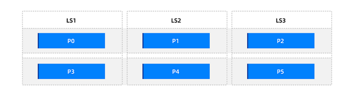
Scenarios:
Scenario 1: Spread a few hot partitions
Suppose only two partitions,
p0andp3, in the partitioned tablet1are hot and need to be spread. Using the principle of the least weight tier, you can apply only one weight tier, i.e., "small weight = 1", to solve this.Set the partition weights to
p0 = 1andp3 = 1. During partition balancing calculations, only these two partitions are balanced; the remaining partitions do not participate and remain balanced by number as much as possible. After partition balancing (either manually triggered or waiting for scheduled balancing), the overall partition distribution is as follows.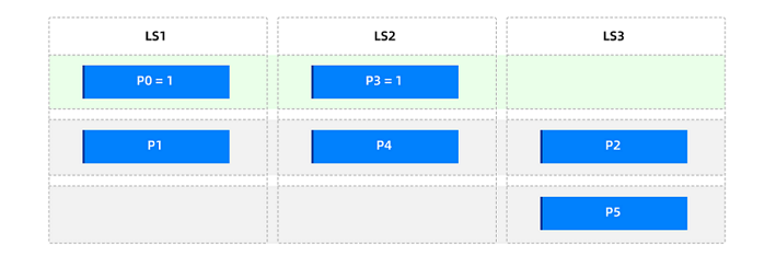
Scenario 2: Distribute all partitions by weight
Assume that among the partitions of the partitioned table
t1, partitionp0receives the most traffic, followed by partitionsp1,p2, andp3, while the traffic of the other partitions is relatively low. If you want to distribute the traffic, you can use the following three weight tiers:Large weight = 100% × Number of partitions in the partitioned table = 6
Medium weight = 50% × Number of partitions in the partitioned table = 3
Small weight = 1
First, set the table-level partition weight to 1, which divides the weight balancing scope to the entire partitioned table. Then, individually set the partition weights to
p0 = 6,p1 = 3,p2 = 3, andp3 = 3. After partition balancing, the overall partition distribution is as follows.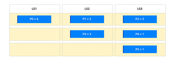
Scenario 3: Balance hot partitions so they are exclusively occupied within their groups
Assume that the traffic distribution among the six partitions in the partitioned table
t1is extremely uneven, with two super-large partitions,p0andp3. You want to prevent other partitions from affecting the read and write operations of these two super-large partitions. You can use the following two weight tiers:Large weight = 100% × Number of partitions in the partitioned table = 6
Small weight = 1
First, set the table-level partition weight to 1, which divides the weight balancing scope to the entire partitioned table. Then, individually set the partition weights to
p0 = 6andp3 = 6. After partition balancing, the overall partition distribution is as follows.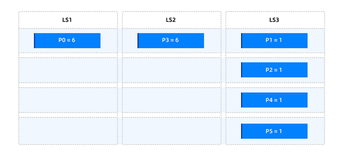
Spread hotspots of non-partitioned tables
For example, assume the following six non-partitioned tables are created with the initial distribution shown below.
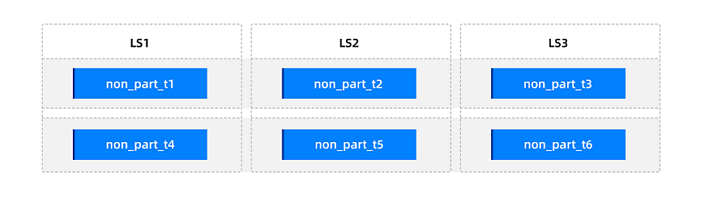
Application scenarios:
Scenario 1: Spread a small number of hotspots
Assume non-partitioned tables
non_part_t1andnon_part_t4are two hotspots on the same log stream that need to be spread. Using the principle of the least weight tier, you can resolve this by using only one weight tier: "Low weight = 1".Set the table-level weights for the non-partitioned tables to
non_part_t1 = 1andnon_part_t4 = 1. After partition balancing, the distribution is as follows.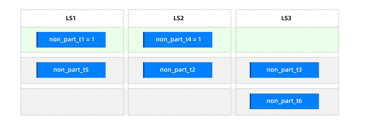
Scenario 2: Distribute by traffic
Assume the traffic for each non-partitioned table is known, with
non_part_t1being the highest, followed bynon_part_t2andnon_part_t3, andnon_part_t4,non_part_t5, andnon_part_t6being the lowest. The goal is to distribute them based on traffic. You can use the following three weight tiers:High weight = 100% * Number of partitions in a partitioned table = 6
Medium weight = 50% * Number of partitions in a partitioned table = 3
Low weight = 1
After setting the corresponding table-level partition weights to
non_part_t1 = 6,non_part_t2 = 3,non_part_t3 = 3,non_part_t4 = 1,non_part_t5 = 1, andnon_part_t6 = 1, the distribution after partition balancing is as follows.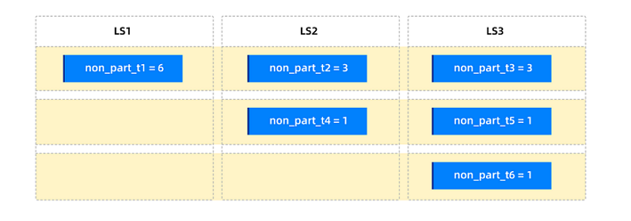
Impact of partition weights on table groups
Tables with partition weights can be added to a table group. For a table group, if there are tables with partition weights within the group, partition balancing will calculate the distribution based on the weighted sum within the partition group. The specific impact of adding tables with partition weights to a table group is shown in the following table.
SHARDING and SCOPE attributes of a table group |
Original partition distribution |
Impact with partition weights |
|---|---|---|
SHARDING = 'NONE' + SCOPE = 'SERVER' |
All Aggregates | No impact |
SHARDING = 'PARTITION' + SCOPE = 'CLUSTER' |
Partitions with identical values within each table's primary partition are aggregated (forming the same partition group), while the primary partitions are scattered. | A small number of weighted partitions can affect the overall distribution of the table group. |
SHARDING = 'ADAPTIVE' + SCOPE = 'CLUSTER' |
|
When all tables in a table group are partitioned into partitions, the distribution of a small number of partitions with weights can affect the overall distribution of the table group. Currently, it is not supported to set partition weights for subpartitioned tables. |
Note
- Table groups with
SHARDING = 'NONE'+SCOPE = 'ZONE'orSHARDING = 'NONE'+SCOPE = 'CLUSTER'do not support partition-level or table-level weights. - Since secondary partition tables do not support setting weights at all, that is, they do not support setting table-level, partition-level, or subpartition-level weights, table groups with
SHARDING = 'SUBPARTITION'+SCOPE = 'CLUSTER'also do not support setting table-level, partition-level, or subpartition-level weights.
Balanced partition count
The goal of balanced partition count is to ensure that the number of partitions of user tables on all log streams (LSs) is evenly distributed (with a deviation of no more than 1).
To achieve this, OceanBase Database uses the concept of "balanced groups" to describe the distribution. Partitions that need to be redistributed are placed into the same balanced group, and balanced partition count is achieved through intra-group balancing and inter-group balancing.
In scenarios without table groups, balanced groups are divided as follows:
Table type |
Balanced Group Partitioning |
Distribution Method (No Table Group) |
|---|---|---|
| Non-partitioned table | All non-partitioned tables in a tenant form a balanced group. | All non-partitioned tables in a tenant are evenly distributed across all LSs of the user (with a deviation of no more than 1). |
| Partitioned table | All partitions in a table form a balanced group. | Each table is divided into partitions, which are evenly distributed across all user-defined logical servers. |
| Subpartitioned table | All subpartitions under each partition of a single table form a balanced group. | All subpartitions under each partition of a single table are evenly distributed across all user-defined LSs. |
During the balancing phase, the system first performs intra-group balancing for all balanced groups, distributing partitions evenly within each group. Then, based on this intra-group balancing, it transfers a portion of partitions from the LS with the most partitions to achieve inter-group balancing, thus achieving balanced partition count.
For example, assume all partitions of four tables are currently on LS1, which are divided into three balanced groups:
Balanced Group 1: non-partitioned tables
non_part_t1andnon_part_t2Balanced Group 2: two partitions of the partitioned table
part_one_t3_p0andpart_one_t3_p1Balanced Group 3: four partitions of the subpartitioned table
part_two_t4_p0s0,part_two_t4_p0s1,part_two_t4_p1s0, andpart_two_t4_p1s1
Initially, the distribution is 8-0-0.
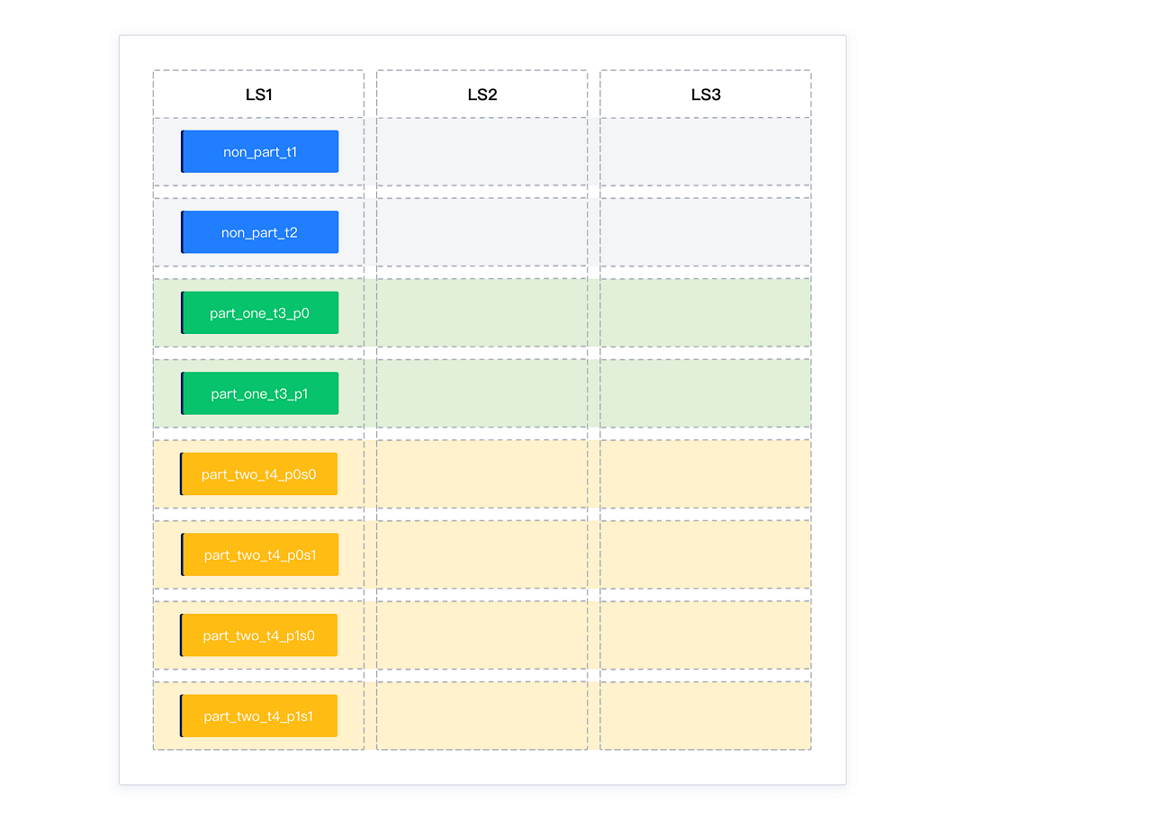
After intra-group balancing, the distribution becomes 4-4-0. Each balanced group is balanced internally, but overall, the distribution is still unbalanced.
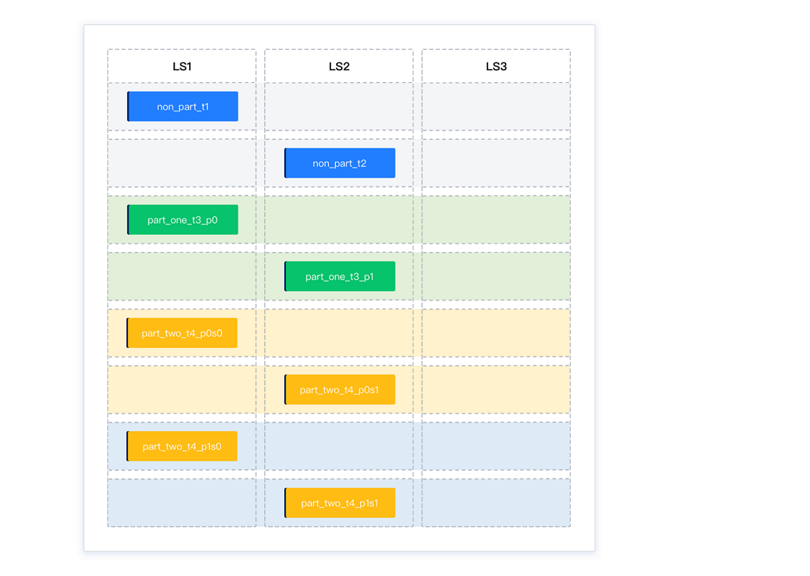
After inter-group balancing, the distribution becomes 3-3-2. One partition is transferred from each of the LSs with the most partitions (LS1 and LS2) to the LS with the fewest partitions (LS3), achieving overall balance.
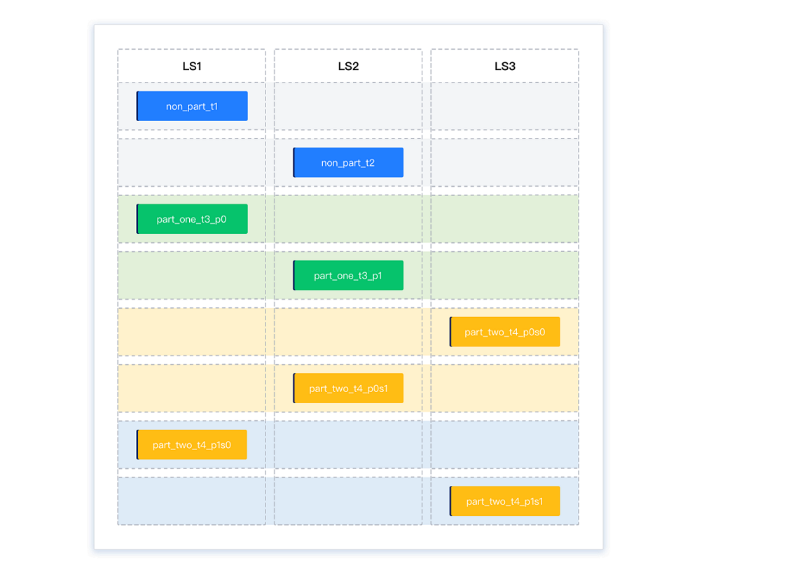
When table groups exist, each table group is an independent balanced group. The system binds the partitions required to be aggregated by the table group and treats them as one partition. Then, it uses the same intra-group balancing and inter-group balancing methods to achieve balanced partition count. When table groups exist, the total number of partitions under a tenant may not be perfectly even.
In scenarios with table groups, balanced groups are divided as follows:
Table type |
Balance group division |
Distribution method |
|---|---|---|
Tables with the Sharding attribute of NONE in a table group |
Form one balance group | All partitions of the table group are distributed on one log stream. |
Partitioned tables with the Sharding attribute of PARTITION or ADAPTIVE in a table group |
All partitions of all tables form one balance group | The partitions of the first table are evenly distributed across all log streams. The partitions of subsequent tables are aggregated with those of the first table. |
Subpartitioned tables with the Sharding attribute of SUBPARTITION in a table group |
All subpartitions under all partitions of all tables form one balance group | Subpartitions with the same partitioning key value under different partitions are bound to the same log stream. |
Subpartitioned tables with the Sharding attribute of ADAPTIVE in a table group |
All subpartitions under all partitions of all tables form one balance group | The subpartitions under each partition of the first table are evenly distributed across all log streams. The subpartitions of subsequent tables are aggregated with those of the first table. |
For example, based on the previous balanced distribution, add a new table group tg1 with SHARDING = 'NONE' + SCOPE = 'SERVER', which contains five non-partitioned tables: non_part_t5_in_tg1, non_part_t6_in_tg1, non_part_t7_in_tg1, non_part_t8_in_tg1, and non_part_t9_in_tg1. Since all tables in tg1 must be bound together, the partition distribution after balancing becomes 4-4-5.
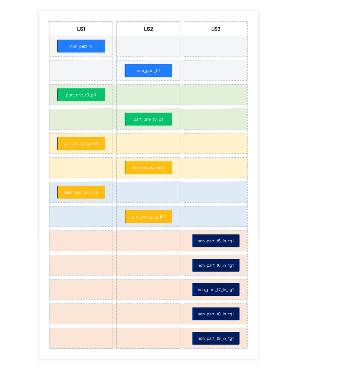
Table groups with SCOPE = 'ZONE'
In the current version, table groups support the SCOPE attribute. The distribution of partitions within a table group is determined jointly by the SHARDING and SCOPE attributes. The SHARDING attribute defines how partitions are aggregated among tables within the table group. A group of aggregated partitions is called a partition group, which is the smallest unit for distribution. The SCOPE attribute determines the distribution scope of all aggregated partition groups within the table group.
Load balancing
For a table group with SCOPE = 'ZONE' (i.e., SHARDING = 'NONE' + SCOPE = 'ZONE'), the number of table groups hosted by each zone is balanced as much as possible. All partitions within a table group are evenly distributed across log streams in the same primary zone using a round-robin method.
The following example illustrates the distribution effect of a table group with SCOPE = 'ZONE'.
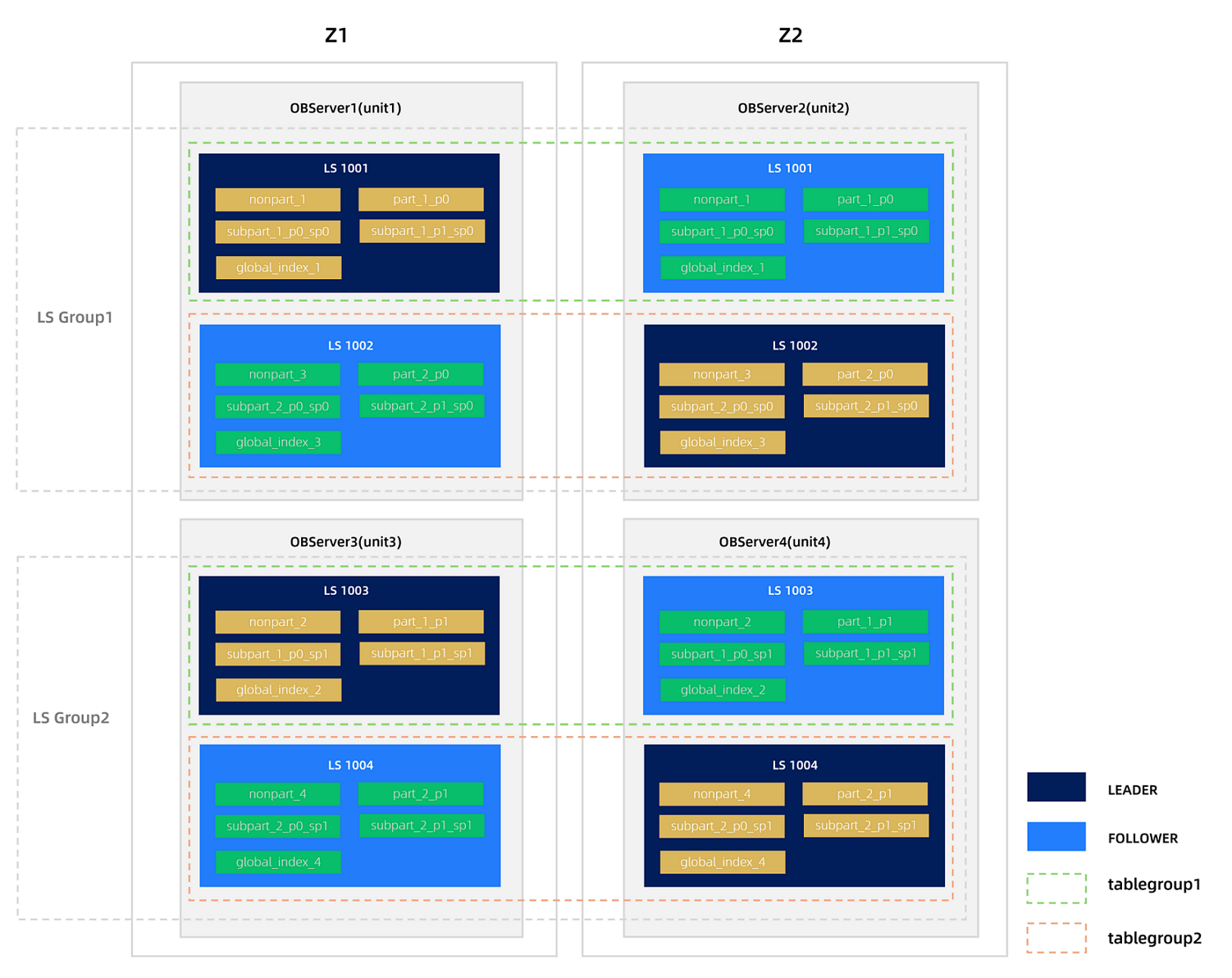
Assume a tenant's locality is FULL{1}@z1, FULL{1}@z2 (2F1A), UNIT_NUM = 2, and PRIMARY_ZONE = 'z1,z2'. The tenant has the following types of tables:
Non-partitioned tables:
nonpart_1,nonpart_2,nonpart_3,nonpart_4Partitioned tables:
part_1,part_2Subpartitioned tables:
subpart_1,subpart_2Global index tables:
global_index_1,global_index_2,global_index_3,global_index_4
Now create two table groups, tablegroup1 and tablegroup2, under the tenant.
obclient> CREATE TABLEGROUP tablegroup1 SHARDING = 'NONE', SCOPE = 'ZONE';
obclient> CREATE TABLEGROUP tablegroup2 SHARDING = 'NONE', SCOPE = 'ZONE';
Then add the corresponding tables and partitions to these two table groups.
obclient> ALTER TABLEGROUP tablegroup1 ADD TABLE nonpart_1,nonpart_2,part_1,subpart_1,global_index_1, global_index_2;
obclient> ALTER TABLEGROUP tablegroup2 ADD TABLE nonpart_3,nonpart_4,part_2,subpart_2,global_index_3, global_index_4;
After partition balancing, the distribution is as follows:
Weight balancing
For a table group with SCOPE = 'ZONE', you can set weights (supported only in MySQL-compatible mode) to ensure that hot table groups are distributed across different zones.
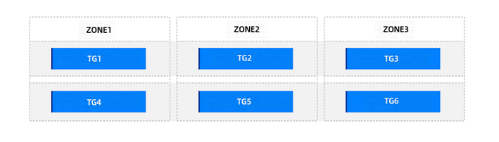
The following example illustrates this. Assume the current tenant has six table groups with SHARDING = NONE and SCOPE = 'ZONE'. The distribution before setting weights is as follows.
Scenario 1: Scattering a small number of hot table groups
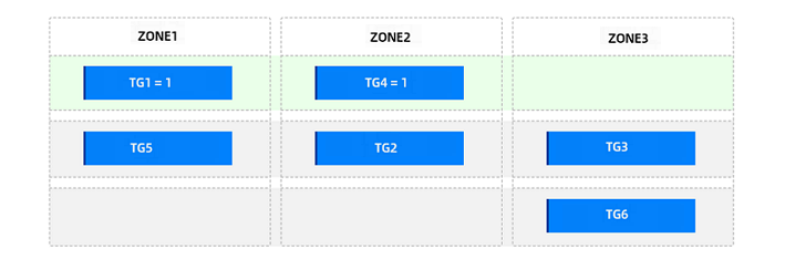
Suppose TG1 and TG4 are two hot table groups in the same zone that need to be scattered. Using the principle of the least weight range, you can resolve this with just one weight range, "Light Weight = 1".
After setting the table group weights to TG1 = 1 and TG4 = 1, the distribution is as follows.
Application scenario 2: Scatter by traffic distribution
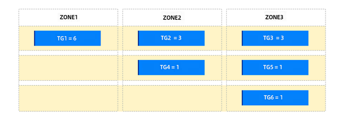
Assume you know in advance the traffic of each table group: TG1 has the highest traffic, followed by TG2 and TG3, and TG4, TG5, and TG6 have the lowest traffic. You want to scatter them based on traffic.
You can use three weight levels:
High weight = 100% * Number of table groups expected to have weights = 6
Medium weight = 50% * Number of table groups expected to have weights = 3
Low weight = 1
After setting the corresponding weights TG1 = 6, TG2 = 3, TG3 = 3, TG4 = 1, TG5 = 1, TG6 = 1, the following distribution is obtained after partition balancing.
Disk balancing
For table groups with SCOPE = 'ZONE', the system automatically attempts to exchange table groups with SCOPE = 'ZONE' across different zones to achieve a balanced total disk usage among zones, while maintaining a balanced number and weights of such table groups per zone.
Table group exchange is initiated only when the total disk usage difference between zones with SCOPE = 'ZONE' table groups meets certain conditions. Both of the following conditions must be met simultaneously:
The total disk usage difference exceeds the total disk usage of the largest zone by
zone_disk_balance_tolerance_percentage/100. The default value is 10%.The tenant-level parameter
zone_disk_balance_tolerance_percentagecontrols the tolerance of the table group disk balancing algorithm for imbalance. Its value range is [0, 100]. A value of100disables disk balancing between zones.The total disk usage of the largest zone exceeds
50 GB * Number of log stream groups.
For the SCOPE = 'ZONE' table groups involved in the exchange, the following additional conditions must also be met:
The weight values of the table groups are the same.
The exchange reduces the disk usage difference between the two zones.
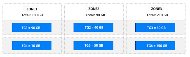
The following example illustrates this. Suppose there are currently six SCOPE = 'ZONE' table groups without assigned weights. After balancing the number of table groups, the distribution is as follows. At this point, ZONE3 has the highest disk usage.
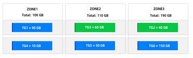
After disk balancing is triggered, the system first exchanges table groups TG3 and TG2 between ZONE3 (with the highest disk usage) and ZONE2 (with the lowest disk usage). The distribution after the exchange is as follows.
Then, it exchanges table groups TG2 and TG4 between ZONE1 and ZONE3. The distribution after the second exchange is as follows.
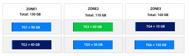
At this point, no further exchanges are possible, and the table group disk balancing ends.
Partition disk balancing
Based on the balance of partition count or partition weight, the load balancing module exchanges partitions as much as possible to ensure that the disk usage difference between log streams does not exceed the percentage set by the cluster-level parameter balancer_tolerance_percentage. If a single partition occupies too much disk space, this balancing effect may not be achieved.
To avoid excessive frequent balancing in scenarios with small data volumes, the current version sets the threshold for partition disk balancing at "50 GB". If the disk usage of a single LS is less than this threshold, disk balancing will not be triggered.
Method for determining partition balancing
Partition balancing refers to the balancing of user tables. You must specify table_type='USER TABLE' when querying. Partition disk balancing is primarily determined by the data_size field in the CDB_OB_TABLET_REPLICAS view.
Query method for partition count balance
obclient [test]> SELECT svr_ip,svr_port,ls_id,count(*) FROM oceanbase.CDB_OB_TABLE_LOCATIONS WHERE tenant_id=xxx AND role='leader' AND table_type='USER TABLE' GROUP BY svr_ip,svr_port,ls_id;Query method for partition disk balance
obclient [test]> SELECT a.svr_ip,a.svr_port,b.ls_id,sum(data_size)/1024/1024/1024 as total_data_size FROM oceanbase.CDB_OB_TABLET_REPLICAS a, oceanbase.CDB_OB_TABLE_LOCATIONS b WHERE a.tenant_id=b.tenant_id AND a.svr_ip=b.svr_ip AND a.svr_port=b.svr_port AND a.tablet_id=b.tablet_id AND b.role='leader' AND b.table_type='USER TABLE' AND a.tenant_id=xxxx GROUP BY svr_ip,svr_port,ls_id;
Scenarios of Aggregation and Disaggregation of Partitions
Partition balancing is a continuous process to dynamically maintain system load balance. In actual business operations, the system aggregates and disaggregates partitions based on real-time load conditions to achieve an optimal balance between resource utilization efficiency and performance. Common scenarios of partition aggregation and disaggregation include:
A tenant undergoes horizontal scaling down and then scaling up. For example, reducing the tenant's
UNIT_NUMfrom N to 1, and then from 1 to N.The number of partitions with the highest priority in a tenant's
PRIMARY_ZONEfirst decreases and then increases. For example, changing the tenant'sPRIMARY_ZONEfromRANDOMtozone1, and then fromzone1back toRANDOM.A large number of tables are added to a table group with a Sharding attribute of
NONE, and then removed from the table group.
Based on existing log stream balancing and partition balancing algorithms, after partition aggregation and disaggregation, consecutive partitions within a partitioned table or non-partitioned tables under the same database might be aggregated onto the same log stream. To address this issue, OceanBase Database has optimized the partition balancing algorithm:
For non-partitioned tables, after aggregation and disaggregation, multiple non-partitioned tables under the same database are dispersed across various user log streams in a balanced manner based on the number of partitions, preventing them from being consecutive on the same log stream.
For partitioned tables, after aggregation and disaggregation, consecutive partitions of the same partitioned table are distributed across various user log streams in a round-robin manner in a balanced number, preventing partitions from being consecutive on the same log stream.